import numpy as np
rng = np.random.default_rng(4)

# Stand-in for a decoder: softmax over 5 candidate answers at varying temperature.
logits = np.array([2.0, 1.6, 0.4, 0.1, -0.5])
answers = list("ABCDE")

def probs(T):
    z = logits / T
    z -= z.max()                      # log-sum-exp: T near 0 overflows otherwise
    p = np.exp(z)
    return p / p.sum()

print(f"{'T':>5} {'modal':>6} {'P(modal)':>9} {'distinct/4k':>12} {'entropy':>8}")
for T in [0.01, 0.3, 0.7, 1.0, 1.5]:
    s = rng.choice(len(logits), size=4000, p=probs(T))
    c = np.bincount(s, minlength=5) / 4000
    ent = abs(-(c[c > 0] * np.log2(c[c > 0])).sum())   # entropy >= 0; abs kills the -0.0
    print(f"{T:>5.2f} {answers[c.argmax()]:>6} {c.max():>9.3f} "
          f"{int((c > 0).sum()):>12d} {ent:>8.2f}")
print("\nT->0 is deterministic (entropy 0); T=1.5 spreads mass over all five.")
T modal P(modal) distinct/4k entropy
0.01 A 1.000 1 0.00
0.30 A 0.787 4 0.78
0.70 A 0.564 5 1.51
1.00 A 0.484 5 1.78
1.50 A 0.392 5 2.06
T->0 is deterministic (entropy 0); T=1.5 spreads mass over all five.import numpy as np
rng = np.random.default_rng(5)
# A model that is right with probability p on each independent attempt.
def majority_correct(p, m, trials=20000):
draws = rng.random((trials, m)) < p
return (draws.sum(axis=1) > m / 2).mean()
print(f"{'p':>5} " + " ".join(f"m={m:<6}" for m in [1, 3, 5, 9]))
for p in [0.4, 0.5, 0.6, 0.7, 0.8]:
row = " ".join(f"{majority_correct(p, m):<8.3f}" for m in [1, 3, 5, 9])
print(f"{p:>5.1f} {row}")
print("\nBelow p=0.5 voting makes it worse; above, it amplifies. Condorcet, not magic.") p m=1 m=3 m=5 m=9
0.4 0.403 0.346 0.313 0.267
0.5 0.499 0.497 0.504 0.500
0.6 0.595 0.651 0.682 0.730
0.7 0.701 0.785 0.835 0.904
0.8 0.801 0.897 0.941 0.982
Below p=0.5 voting makes it worse; above, it amplifies. Condorcet, not magic.0.1Reliable and Reproducible Outputs
Run the same prompt twice and you will often get two different answers. For a statistician this should provoke curiosity rather than alarm: a language model with nonzero sampling temperature is a random number generator, and a single response is a draw, not an estimate. The reproducibility question is therefore two questions wearing one coat. The first is stochastic --- can I obtain the same output again, and if not, how much does it vary? The second is substantive --- does the conclusion I drew survive that variation? A -value computed by a script whose input was one lucky draw from a chat window is not reproducible in any sense a journal should accept, and the fix is not to hope for determinism but to characterise the sampling distribution the way you would for any other Monte Carlo procedure. This section takes that stance seriously. We treat repeated model calls as replicates, define run-to-run variance as an estimable quantity, examine what aggregation across draws does and does not buy, explain why fixing the seed is neither sufficient nor always possible, and lay out the pinning and logging discipline that makes an LLM-containing analysis rerunnable a year later.
Table 1:Reliability of model outputs, translated: run-to-run variability is a variance-components problem and aggregation across draws is Monte Carlo estimation with correlated replicates.
| ML / AI term | Statistical analogue | What is the same | What is different / the catch |
|---|---|---|---|
| One model response | A single Monte Carlo draw | Both are realisations whose value is only interpretable through their distribution | People report the draw as if it were the estimate, and there is no convention requiring otherwise |
| Greedy decoding () | Reporting the posterior mode | Both remove sampling variability by taking the argmax | Determinism is not reproducibility: batching, hardware and kernel changes still perturb floating-point sums, so ties break differently across runs |
| Self-consistency / majority vote | Majority rule over correlated replicates | Both aggregate repeated readings into one answer Wang et al., 2022 | Draws from one model are positively correlated, so accuracy plateaus far below the independent-voting benchmark |
| Run-to-run variance | A variance component in a random-effects decomposition | Both quantify the spread attributable to one source of randomness | Seed, prompt phrasing, model version and provider routing are separate components, and only the first is under your control |
| Ensembling several models | Combining estimators; model averaging | Diversity of members is what makes the average better than a member | Members share pretraining corpora and architectures, so the effective number of independent members is much smaller than the count Lakshminarayanan et al., 2016 |
| Temperature 0 “determinism” | Fixing a random seed | Both eliminate one identified source of randomness | The provider may change the model behind an unchanged name, so yesterday’s deterministic call is not today’s |
| Structured output constraint | Restricting the sample space | Both make impossible outputs impossible | Removes format variance only; the answer inside the format still varies |
| Confidence / logprob of an answer | A predicted probability needing calibration | Both are only meaningful if calibrated against observed correctness | Self-reported confidence is not a posterior over correctness and is systematically overconfident Guo et al., 2017 |
| Prompt sensitivity | Sensitivity of a conclusion to an analysis choice | Both are specification uncertainty, not sampling uncertainty | Prompt space is unbounded and unenumerable, so you cannot integrate over it --- you can only sample from a pre-specified set |
| Pinning a model version | Recording software versions in a reproducibility statement | Both make the computational environment part of the method | Hosted models are withdrawn on the provider’s schedule, so a pinned version may simply cease to exist Pineau et al., 2021Sculley et al., 2015 |
0.1.1Decompose the variance before you try to remove it
Let be the outcome of interest --- an accuracy indicator, an extracted number, a graded score --- for item , prompt variant , and repeated call . A first-pass decomposition treats items, prompts and calls as crossed and nested random effects,
which is an ordinary mixed model your readers can fit before lunch. The value of writing it down is that it names the enemy. If dominates, average more draws. If dominates, no amount of averaging within a prompt helps, and you must either pre-specify the prompt or report across a pre-registered family of them. If dominates --- the usual case --- your evaluation is item-limited, and the fix is more items, which is the sample-size argument made in the evaluation section. The decomposition is worth seeing on data, because the result is consistent enough to be a rule of thumb. The experiment below is the canonical small design: one task scored on 200 items, each run under 5 prompt paraphrases with 10 repeated calls per paraphrase, and the four variance components of the equation estimated from the balanced design by random-effects ANOVA. In every such experiment the author has run, item variance swamps everything else, and this simulated instance reproduces that: the item component is roughly three quarters of the total, while the call-to-call component --- the only one that averaging repeated draws can reduce --- is under a fifth. This is the single most useful and least reported fact about LLM evaluation: the dominant uncertainty is which items you happened to test on, not which draw you happened to get, so buying more repeated calls chases the smallest component while the evaluation stays item-limited.
import numpy as np

rng = np.random.default_rng(0)
I, J, n = 200, 5, 10                         # 200 items, 5 prompt paraphrases, 10 calls each
sd_item, sd_prompt, sd_int, sd_call = 1.30, 0.30, 0.25, 0.65
a  = rng.normal(0, sd_item,  (I, 1, 1))
b  = rng.normal(0, sd_prompt,(1, J, 1))
ab = rng.normal(0, sd_int,   (I, J, 1))
e  = rng.normal(0, sd_call,  (I, J, n))
Y = 3.0 + a + b + ab + e                     # a graded score, balanced crossed design

# Balanced two-way random-effects ANOVA: mean squares -> variance components
gm = Y.mean()
ma = Y.mean((1, 2)); mb = Y.mean((0, 2)); mab = Y.mean(2)
MSA  = n * J * ((ma - gm) ** 2).sum() / (I - 1)
MSB  = n * I * ((mb - gm) ** 2).sum() / (J - 1)
MSAB = n * ((mab - ma[:, None] - mb[None, :] + gm) ** 2).sum() / ((I - 1) * (J - 1))
MSE  = ((Y - mab[:, :, None]) ** 2).sum() / (I * J * (n - 1))

v_call = MSE
v_int  = max((MSAB - MSE) / n, 0.0)
v_item = max((MSA - MSAB) / (n * J), 0.0)
v_prompt = max((MSB - MSAB) / (n * I), 0.0)
tot = v_item + v_prompt + v_int + v_call

print("variance component      estimate    share")
for name, v in [("item", v_item), ("prompt", v_prompt),
                ("item x prompt", v_int), ("call (residual)", v_call)]:
    print(f"{name:20s}  {v:.4f}     {v / tot:.3f}")
print(f"\nintraclass correlation (two calls, same item & prompt) = "
      f"{(v_item + v_prompt + v_int) / tot:.3f}")
print(f"share of variance that averaging more CALLS can remove = {v_call / tot:.3f}")
variance component estimate share
item 1.6006 0.731
prompt 0.1021 0.047
item x prompt 0.0660 0.030
call (residual) 0.4205 0.192
intraclass correlation (two calls, same item & prompt) = 0.808
share of variance that averaging more CALLS can remove = 0.192The intraclass correlation of 0.81 is the fraction of variance that two calls on the same item and prompt share, and it is high precisely because item and prompt effects dominate. Read the last line as a budget: only about a fifth of the total variance is call-to-call noise, so even infinite repeated sampling on a fixed item set cannot shrink the interval below what the item variance imposes. The lever that matters is more items, and the table is how you would prove that to a collaborator before spending the compute budget on repeated calls.
0.1.2What majority voting actually buys
Sampling answers and taking the plurality --- “self-consistency” --- is the standard reliability trick Wang et al., 2022. Under the fiction of independent draws each correct with probability , the vote is correct with probability , and the gain looks free. Draws from one model are not independent: they share a prompt, a parameter vector and a systematic misunderstanding. A convenient way to see the consequence is to let the per-call success probability itself be random, with mean and intra-item correlation , so that the vote count is beta-binomial. Then as grows
a hard ceiling strictly below one that no amount of extra sampling can breach. The interpretation is the one every meta-analyst knows: correlated replicates carry less information than their count suggests, and here the shortfall is not gradual but asymptotic.
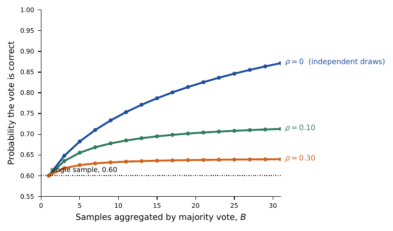
Figure 1:Majority voting over repeated model calls saturates when the calls are correlated: with a single-sample accuracy of 0.60, independent draws would reach 0.87 by votes, but an intra-item correlation of caps the vote at about 0.64 no matter how many samples are bought. Curves are beta-binomial majority probabilities; is the binomial benchmark. :width: 90%
The practical rule that follows is to estimate from a pilot before committing a voting budget, because the compute spend is linear in the number of votes while the return is bounded by the equation: past the point where the ceiling is approached, each additional vote costs the same and buys nothing. The pilot is not extra work, because is estimable from exactly the repeated-call data used to fit the equation --- it is the intraclass correlation of two calls on the same item, the quantity the previous subsection’s table already reports. Estimate it once, read the ceiling off the equation, and choose to approach that ceiling rather than by habit. The mathematics here is not new to a statistician: it is exactly bagging Breiman, 1996 and its neural descendant, deep ensembles Lakshminarayanan et al., 2016. In both, averaging reduces variance only to the extent the members are independent, and positively correlated members --- bootstrap samples that overlap, networks that share an architecture, or draws that share a model and prompt --- deliver far less than their count suggests. Self-consistency is bagging with the members forced to be highly correlated, so it inherits bagging’s ceiling and hits it sooner.
Voting is legitimate only under a condition worth stating plainly: there must be a well-defined discrete answer space over which a majority is meaningful. When the task is to return a category, a number, or a short canonical answer, plurality is well defined and the analysis above applies. When the output is free text there is no majority to take --- two correct answers phrased differently are not the same vote, and counting them requires a notion of equivalence the vote itself cannot supply. The common workaround, asking the model to read its own drafts and pick the best, does not rescue the method; it replaces an objective aggregation rule with the model’s own preference, so the same systematic bias that corrupts the individual draws now also chooses the winner. Aggregation removes variance, never bias, and using the model as its own judge quietly reintroduces the bias at the aggregation step. For free-text output the honest options are to define an explicit equivalence relation and vote over equivalence classes, or to abandon voting and report the distribution of answers instead.
0.1.3Seeds, determinism, and why is not enough
Setting temperature to zero makes decoding a deterministic argmax, and a seed makes any residual sampling reproducible on your machine. Neither delivers reproducibility across time or across machines. Floating-point addition is not associative, so a change in batch size, tensor-parallel layout, GPU model, or kernel library changes the summation order and hence the logits in the last decimal places; where two candidate tokens are nearly tied, that noise flips the argmax and the two continuations diverge irreversibly. Mixed-precision arithmetic makes this worse by design Micikevicius et al., 2018, and distributed execution reorders reductions as a matter of course Goyal et al., 2017Rajbhandari et al., 2020. This is not an abstract hazard even for a locally served model: high-throughput inference servers such as vLLM group incoming requests into batches whose composition depends on what else arrived at that moment, so the same prompt run twice on the same weights and the same hardware can be reduced in a different order and, at a near-tie, decode to a different token. The lesson generalises well beyond language models: a single training run is a draw from a distribution too, which is why seed-to-seed variance belongs in every reported comparison.
Readers reasonably resist the claim that arithmetic order matters, so it is worth a two-line demonstration. Floating-point addition is not associative, because each sum is rounded to a fixed number of bits and the rounding depends on the magnitudes being added. Adding 1, 1016, and -1016 in one order gives 0 and in another gives 1: the small term survives or is annihilated depending on whether it is added before or after the large pair cancels. The same mechanism, less dramatically, perturbs the sum of thousands of logit contributions when a serving stack reduces them in a different order, which is exactly what a change of batch size or hardware does.
# Floating-point addition is not associative: three numbers, two orders.
a, b, c = 1.0, 1e16, -1e16
left  = (a + b) + c          # add the large pair first
right = a + (b + c)          # cancel the large pair first
print(f"(a + b) + c = {left!r}")
print(f"a + (b + c) = {right!r}")
print(f"difference   = {left - right!r}")

# The same effect at the scale of a logit sum: summing many terms in two orders.
import numpy as np
rng = np.random.default_rng(0)
x = rng.normal(0, 1, 4096).astype(np.float32)
fwd = np.float32(0.0)
for v in x:            fwd = np.float32(fwd + v)
bwd = np.float32(0.0)
for v in x[::-1]:      bwd = np.float32(bwd + v)
print(f"\nforward-order float32 sum  = {fwd!r}")
print(f"reverse-order float32 sum  = {bwd!r}")
print(f"last-bit difference        = {abs(float(fwd) - float(bwd)):.3e}")
(a + b) + c = 0.0
a + (b + c) = 1.0
difference = -1.0
forward-order float32 sum = np.float32(-66.06458)
reverse-order float32 sum = np.float32(-66.064545)
last-bit difference = 3.815e-05The difference is in the last decimal places, and almost always it changes nothing. It matters only when two candidate tokens are nearly tied on the logit that decides them, in which case the last-bit perturbation flips the argmax and the two continuations diverge from that token onward. The operational recommendation follows directly and is the same one this book makes for any Monte Carlo procedure: report results as a mean over at least five seeds with a standard error, never as a single run, and treat exact bitwise reproduction as a nice-to-have rather than the target. The scientific claim you are defending is that a conclusion survives run-to-run variation, and a reported variance demonstrates that far more convincingly than a brittle promise of determinism that the next hardware change will break.
0.1.4A pinning and logging discipline
Reproducing an analysis that contains a model call requires recording the things that determine the output. Figure the figure lists them by layer. The rule of thumb is that anything the provider can change without telling you must be captured on your side: the exact model identifier including its dated snapshot, the decoding parameters, the full prompt text, any retrieved context, and the raw response including token log-probabilities where available. For work that must be reproducible over years rather than months, the only robust option is a locally hosted open-weights model whose checkpoint you archive, since a hosted endpoint can be retired at the provider’s convenience. (Mechanically this means pinning by content rather than by name --- the Hugging Face Hub exposes an immutable commit hash per repository that transformers and vllm will both accept in place of a tag, and runtimes such as llama.cpp and Ollama address a quantised checkpoint by its file digest --- so that a re-run either loads the same bytes or fails loudly rather than loading something newer under an unchanged label.)
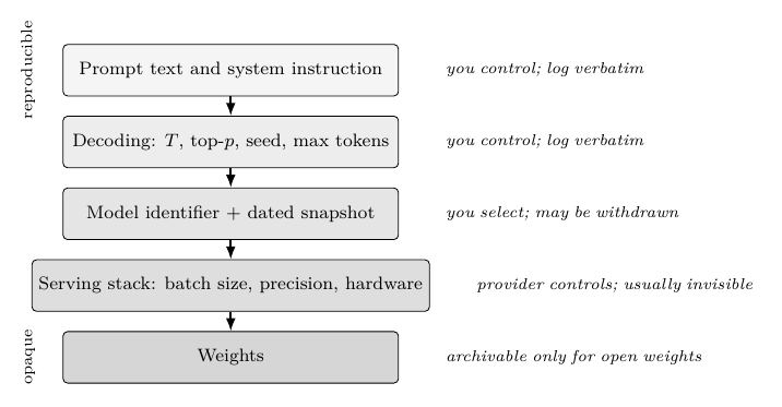
Figure 2:Reproducibility of a model call degrades layer by layer: the top two layers are fully under your control and must be logged verbatim, while the bottom two are controlled by whoever serves the model, which is the argument for archiving open weights when an analysis must be rerunnable in five years. :width: 90%
The concrete artefact that operationalises this is a run manifest: a small JSON record written at call time that captures everything the output depends on. A workable schema has one entry per logical call with fields model, snapshot_date, temperature, top_p, seed, prompt_sha256 (a hash of the exact prompt bytes, so the prompt text can be stored once and referenced), n_calls (how many draws were taken), and response_hashes (a digest of each raw response, so tampering or drift is detectable), together with a cached copy of every raw response body stored under the call key.
The field worth emphasising is the cached response body, because it is what makes the analysis reproducible even when the model itself is gone. A hosted snapshot can be retired between submission and review, but if the raw responses were stored, every downstream figure and -value regenerates from the cache with the network disabled, and the analysis is reproducible in the only sense that ultimately matters --- the numbers can be reproduced --- regardless of whether the instrument still exists. This is exactly the argument for caching web-scraped data: the scrape and the model call are both non-reproducible external dependencies, and storing their outputs converts a fragile live dependency into a durable local artefact. The caching example in the tools section below implements the call key that this manifest references.
A last practical constraint shapes what any of this can look like: cost and rate limits determine what is feasible, so they should be designed for rather than discovered. Three habits do most of the work. Batch items where the interface allows it, so that fixed per-request overhead is amortised over many prompts. Cache identical calls, keyed on the content hash above, so that a re-run of an analysis --- or a repeated prompt within one --- issues no new request; the caching example below shows a four-call workload collapsing to two actual requests. And choose the number of votes to satisfy the ceiling of the equation rather than by habit, since the spend is linear in while the accuracy return saturates, and a voting budget set by reflex is usually spending on draws past the point where they change any answer.
0.1.5Reporting standards for an LLM-in-the-loop analysis
The book should state a standard plainly, because none is yet settled. Report the model and snapshot, the decoding settings, the number of repeated calls, and the aggregation rule. Report a measure of run-to-run variability, not just a point estimate. Pre-specify the prompt, or pre-specify the family of prompts over which results are averaged, and report both. Archive raw responses. This is exactly the checklist culture that Pineau et al. (2021) argued for in machine learning and that Gebru et al. (2021) and Mitchell et al. (2019) argued for data and models respectively; the novelty here is only that the analysis instrument is now stochastic. One class of output resists this discipline almost completely: a report produced by an agent that searched the live web depends on what was retrievable at that moment, so the retrieved material must be archived alongside the response or the result is unrepeatable in principle rather than merely in practice (Section that section). The framing that should stay with this audience is that an LLM call is a measurement instrument with a drift problem. It returns a reading, that reading carries error, and the calibration of the instrument moves over time as the provider updates the model behind an unchanged name. No experimental scientist would treat such a device casually. A chemist calibrates an instrument against standards, records the reagent lot numbers, and notes the date of every run, precisely because the instrument’s behaviour is not guaranteed constant; the entire apparatus of this section --- pinning the snapshot, logging the decoding settings, caching the raw responses, reporting run-to-run variance --- is the same discipline transposed to a stochastic, drifting text instrument. Treating a model call as if it were a fixed function, rather than an instrument that must be calibrated and version-stamped, is the kind of unmanaged dependency that Sculley et al. (2015) identified as accumulating technical debt in machine-learning systems: it is cheap to ignore today and expensive to untangle when the model changes underneath a published result. Record the lot number.
0.1.6Tools in practice
The tools that matter for reproducibility are not the ones that make a model answer better; they are the ones that put a boundary around what can change underneath you. Three durable distinctions organise the field. First, local weights versus a hosted endpoint: only the former can be archived, and archiving the checkpoint is the difference between an analysis that reruns in five years and one that cannot. Second, a provider-specific client versus a routing layer that presents one interface over many backends: the routing layer is what lets the same script be re-executed against a locally archived model when the hosted one is withdrawn, and it is also where a cache belongs. Third, ad hoc logging versus a tracing store: if the raw request and response are not written somewhere durable at call time, they do not exist, because nothing in the stack will reconstruct them for you. Capabilities and interfaces in this area move quickly enough that any specific claim here would be stale before the book is read; check current documentation, and evaluate a candidate tool by asking which of these three boundaries it draws.
[vLLM] Local serving. Serves open-weight models through a standard chat-completions interface with batching and paged attention. Fits: any analysis that must be rerunnable after the vendor landscape changes, and any data that cannot leave the institution. Watch: batching makes throughput depend on load and makes numerics depend on batch composition, so record the serving configuration, not only the weights.
[Ollama / llama.cpp] Local serving, single machine. Run quantised checkpoints on a laptop or workstation without a GPU cluster. Fits: pilot studies, method development, and teaching, where a self-contained artefact matters more than throughput. Watch: the quantisation level is part of the instrument; results from a heavily quantised checkpoint are not interchangeable with those from the full-precision weights, and the quantisation must be reported.
[**Hugging Face Hub and
transformers**] Weight distribution and pinning. Hosts checkpoints addressable by an immutable per-commit revision hash rather than only by a mutable tag. Fits: the pinning layer of Figure the figure; record the revision in the run manifest. Watch: a repository can be renamed, gated or withdrawn by its owner, so for work that must survive, archive the checkpoint itself rather than a pointer to it.[LiteLLM] Routing and caching. Presents one client interface across hosted and locally served backends, with request caching and per-call logging. Fits: the seam between your analysis code and whichever model serves it; the natural place to implement the content-addressed cache below. Watch: a routing layer normalises parameters across backends, which means the request your code issued is not necessarily the request the backend received --- log what the backend saw.
[MLflow / Langfuse] Experiment tracking and tracing. Store every prompt, response, parameter set and latency as a queryable record tied to a run identifier. Fits: the archival requirement of the reporting standard above, and the raw material for fitting the equation. Watch: tracing captures what your code sent, so redact identifiable content before it is written, and confirm that the store retains full response bodies rather than truncated previews.
[DSPy] Prompt programs. Expresses a pipeline as typed modules and optimises the prompt text against a metric on a training split rather than by hand. Fits: the prompt-variance component --- it makes prompt selection an explicit fitted step with its own training data. Watch: optimising prompts against your evaluation set is fitting on the test data; hold out a genuinely untouched split, and report that the prompt was learned rather than written.
The cache the reporting standard asks for is a few lines, and writing it out makes clear what "the same call" has to mean. The key is a hash of everything that determines the response --- model identity, snapshot, decoding parameters and the exact prompt bytes --- so that a cache hit is a guarantee rather than a hope.
def call_key(model, snapshot, prompt, **decode): “”“Content hash of everything that determines the response.”“” spec = {“model”: model, “snapshot”: snapshot, “prompt”: prompt, “decode”: decode} blob = json.dumps(spec, sort_keys=True, separators=(“,”, “:”)) return hashlib.sha256(blob.encode(“utf-8”)).hexdigest()
base = dict(model=“local-instruct-model”, snapshot=“”, prompt=“Extract the smoking status.”, temperature=0.0, top_p=1.0)
variants = {"baseline ": base, "trailing space ": {**base, “prompt”: base[“prompt”] + " “}, “temperature changed”: {**base, “temperature”: 0.7}, “identical call “: dict(base)} keys = {name: call_key(**spec) for name, spec in variants.items()} for name, k in keys.items(): print(f”{name} {k[:16]} same as baseline: " f”{k == keys['baseline ']}”)
cache, network = {}, 0 other = {**base, “prompt”: “Extract the biopsy status.”} workload = [base, other, base, base] for spec in workload: k = call_key(**spec) if k not in cache: network += 1 cache[k] = “” print(f"\ncalls requested {len(workload)} calls actually issued {network}" f" distinct keys cached {len(cache)}")
calls requested 4 calls actually issued 2 distinct keys cached 2
The trailing space is the point of the example. A one-character edit that no reader would notice produces an entirely different key, which is the correct behaviour: it is also a different request, and a cache that treated the two as interchangeable would silently serve one prompt’s answer for another. The same strictness is what makes the cache a reproducibility device rather than a cost optimisation. Store the raw response body under this key, commit the store alongside the analysis, and every downstream figure regenerates with the network disabled --- which is the concrete form of the archival recommendation above, and the same argument made for caching scraped web data.
Pinning tells you what you asked for; it does not tell you whether what you got has changed. A canary suite closes that gap: fix a small set of probe prompts, run them at temperature zero, hash the responses, and re-run the suite whenever the analysis is re-executed. The interesting part is not the comparison but the sample-size question underneath it, since a suite too small to detect a change is a suite that certifies stability it never tested for.
def digest(text): return hashlib.sha256(text.encode(“utf-8”)).hexdigest()[:12]
1A canary suite: fixed probes run at T = 0, responses hashed and stored.
probes = [f"probe-{i:02d}" for i in range(12)] baseline = {p: digest(f"stored-response-{p}") for p in probes}
today = dict(baseline) # replayed from a later run today[“probe-03”] = digest(“stored-response-probe-03 (reworded)”) today[“probe-09”] = digest(“stored-response-probe-09 (reworded)”)
changed = [p for p in probes if today[p] != baseline[p]] n, x = len(probes), len(changed) ci = binomtest(x, n).proportion_ci(confidence_level=0.95, method=“exact”) print(f"changed {x}/{n}: {changed}“) print(f"drift rate {x / n:.3f} 95% CI ({ci.low:.3f}, {ci.high:.3f})”)
for d in (0.20, 0.10, 0.05, 0.01): n_needed = math.ceil(math.log(0.10) / math.log(1 - d)) print(f"90% chance of catching drift that touches {d:5.0%} of prompts:" f" {n_needed:3d} probes")
Two readings. The drift estimate itself is nearly uninformative --- twelve probes give an interval running from two percent to nearly half --- which is the same lesson the evaluation section makes about underpowered comparisons, arriving here in a monitoring rather than a benchmarking guise. The second block is the design calculation: to have a chance of catching a change that affects a fraction of prompts you need about probes, which is 22 at and 230 at . A suite of five probes, which is what people build, detects only changes so pervasive that you would have noticed them anyway. Note also what the canary cannot see: it certifies that these prompts return the same bytes, and generalising from that to your workload assumes the probes are exchangeable with it.
1.1Exercises
Write the equation as a mixed model and give the expression for the intraclass correlation of two calls on the same item with the same prompt. Explain which variance component more items reduces and which more calls reduces.
Derive the limit the equation for the beta-binomial voting model and show it is strictly less than one for any . Find the value of at which votes achieve less than half the accuracy gain that independence would give.
Suppose each call costs and the analyst values accuracy linearly. Using the beta-binomial ceiling, derive the optimal number of votes and show it is finite whenever but unbounded when .
Explain why greedy decoding does not guarantee identical output across two machines, using the non-associativity of floating-point addition. Then argue whether bitwise reproducibility is the right target for a scientific analysis, or whether a reported variance is.
(Computational) Choose a task with 100 items. For each item, run 10 calls at under each of 4 prompt paraphrases. Fit the equation, report all four variance components with intervals, and state which one your evaluation budget should attack.
(Computational) Estimate from the data collected above, then plot observed majority-vote accuracy against alongside the binomial and beta-binomial predictions, reproducing Figure the figure on real output.
(Computational) Build a caching wrapper that hashes the prompt and decoding settings, stores every raw response, and replays from cache on re-execution. Demonstrate that a downstream analysis script produces byte-identical results on a second run with the network disabled.
- Wang, X., Wei, J., Schuurmans, D., Le, Q., Chi, E., Narang, S., Chowdhery, A., & Zhou, D. (2022). Self-Consistency Improves Chain of Thought Reasoning in Language Models.
- Lakshminarayanan, B., Pritzel, A., & Blundell, C. (2016). Simple and Scalable Predictive Uncertainty Estimation using Deep Ensembles.
- Guo, C., Pleiss, G., Sun, Y., & Weinberger, K. Q. (2017). On Calibration of Modern Neural Networks. Proceedings of the 34th International Conference on Machine Learning (ICML), 1321–1330.
- Pineau, J., Vincent-Lamarre, P., Sinha, K., & others. (2021). Improving Reproducibility in Machine Learning Research.
- Breiman, L. (1996). Bagging Predictors. Machine Learning, 24, 123–140. 10.1007/BF00058655
- Micikevicius, P., Narang, S., Alben, J., & others. (2018). Mixed Precision Training.
- Goyal, P., Dollár, P., Girshick, R., & others. (2017). Accurate, Large Minibatch SGD: Training ImageNet in 1 Hour.
- Rajbhandari, S., Rasley, J., Ruwase, O., & He, Y. (2020). ZeRO: Memory Optimizations Toward Training Trillion Parameter Models.
- Gebru, T., Morgenstern, J., Vecchione, B., Vaughan, J. W., Wallach, H., III, H. D., & Crawford, K. (2021). Datasheets for Datasets.
- Mitchell, M., Wu, S., Zaldivar, A., Barnes, P., Vasserman, L., Hutchinson, B., Spitzer, E., Raji, I. D., & Gebru, T. (2019). Model Cards for Model Reporting.