import json

SCHEMA = {"study_id": str, "n_participants": int, "effect": float, "outcome": str}

candidates = [
    '{"study_id": "S1", "n_participants": 240, "effect": 0.31, "outcome": "mortality"}',
    '{"study_id": "S2", "n_participants": "two hundred", "effect": 0.4, "outcome": "mortality"}',
    '{"study_id": "S3", "n_participants": 88, "effect": 0.12}',
    '```json\n{"study_id": "S4", "n_participants": 51, "effect": 0.9, "outcome": "LOS"}\n```',
]

def parse(raw):
    s = raw.strip()
    if s.startswith("```"):                       # models love fencing their JSON
        s = "\n".join(l for l in s.split("\n") if not l.startswith("```"))
    try:
        obj = json.loads(s)
    except json.JSONDecodeError as e:
        return None, f"unparseable: {e.msg}"
    missing = [k for k in SCHEMA if k not in obj]
    if missing:
        return None, f"missing fields: {missing}"
    for k, typ in SCHEMA.items():
        if typ is float and isinstance(obj[k], int):
            obj[k] = float(obj[k])
        elif not isinstance(obj[k], typ):
            return None, f"field {k!r} is {type(obj[k]).__name__}, expected {typ.__name__}"
    return obj, "ok"

for raw in candidates:
    obj, msg = parse(raw)
    tag = obj["study_id"] if obj else "--"
    print(f"{tag:<4} {msg}")
S1 ok
-- field 'n_participants' is str, expected int
-- missing fields: ['outcome']
S4 ok0.1Data Extraction
A great deal of the world’s scientific information is locked in prose: clinical notes, pathology reports, published tables, protocol documents, free-text survey responses, and the methods sections of ten thousand papers you would like to meta-analyse. Language models are startlingly good at turning that prose into a rectangular data frame, and this is arguably their highest-value application in research --- it converts a task that used to cost months of trained abstractor time into an afternoon of compute. It is also the application where a statistician’s instincts pay off fastest, because the output of an extraction pipeline is not data. It is a measurement of data, with a sensitivity, a specificity, and an error process that will propagate into every estimate computed downstream. The central message of this section is that this problem has been solved before, under different names: measurement error, misclassification, and two-phase sampling with a validation subsample. If you extract a variable with accuracy and then regress an outcome on it as though it were observed, you have not produced a slightly noisy estimate; you have produced a systematically attenuated one, and you can say by how much.
Table 1:LLM-based extraction is a measurement-error problem in disguise; each row names the classical machinery that already handles it.
| ML / AI term | Statistical analogue | What is the same | What is different / the catch |
|---|---|---|---|
| Information extraction / structured output | Measurement of a latent variable with error | Both produce a surrogate for an unobserved truth ; both need the error distribution to be usable | The error process is a black box that can change without warning when the model version changes, so the measurement instrument is not stable over time |
| Extraction accuracy | Sensitivity and specificity of a classifier | The table is the same table | A single “accuracy” number hides the sens/spec split, and only the split determines the direction and magnitude of downstream bias |
| Human-labelled gold standard | Validation subsample in a two-phase design | Both let you estimate the measurement-error model and correct for it | Gold labels are expensive and themselves imperfect; inter-rater disagreement puts a ceiling on measurable accuracy |
| Non-differential extraction error | Misclassification independent of the outcome | Both give the classical attenuation-toward-null result | If the model reads outcome-related cues in the same note, the error becomes differential and the bias can go in either direction, including away from the null |
| Structured/JSON-constrained decoding | Restricting the parameter space; a constrained estimator | Both eliminate a class of impossible outputs by construction | It guarantees the output parses, not that it is correct; a schema-valid wrong value looks exactly like a right one |
| Confidence score / logprob of an extracted field | A predicted probability requiring calibration | Both are only useful if | Model confidence is systematically overconfident and must be recalibrated on a labelled set before it can be used for triage Guo et al., 2017 |
| Abstain / route-to-human threshold | A decision rule with an indifference region | Both trade coverage against precision through a cut-point on a score | The abstention rate is not missing at random: the model abstains on the hardest, most atypical records, which are often the interesting ones |
| Self-consistency voting | Majority rule over correlated raters | Both aggregate votes into a single reading | Correlation among draws caps the achievable accuracy far below the independent -voting benchmark |
| Retrieval over a document corpus | Sampling frame construction | Both determine which units are eligible to contribute data | Documents that retrieval fails to surface are missing from the frame entirely, and that missingness correlates with document length and vocabulary |
| Regression on extracted variables | Regression with a mismeasured covariate | Both need a correction: regression calibration, SIMEX, or multiple imputation Carroll et al., 2006 | Naive analysis is not conservative in general; with several mismeasured covariates the bias in any one coefficient can be in either direction |
0.1.1The pipeline, and where the statistics enter
An extraction pipeline has five stages: acquire documents, segment them into passages, prompt a model for a structured record, validate the record against a schema, and then analyse. Figure the figure draws it with the validation subsample entering where it belongs --- as a designed second phase, not as a spot check bolted on at the end. The single most consequential design decision is to reserve labelling effort for a random validation sample rather than spending all of it on prompt iteration, because the validation sample is what converts an unquantified pipeline into a measurable one. The acquisition stage is usually a document-conversion problem before it is a language problem (GROBID turns scholarly PDFs into structured TEI with the reference list and section boundaries already delimited, and general layout converters such as Docling or Marker do the same job for reports and forms), and where the corpus must itself be assembled by an agent that searches and synthesises, the verification machinery of Section that section applies to the corpus before any extraction runs on it.
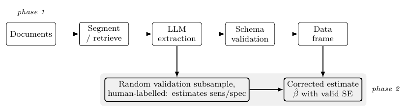
Figure 1:Treat extraction as a two-phase design: the model reads every document, a random subsample is also read by a human, and the subsample identifies the measurement-error model that corrects the final estimate. :width: 90%
How large should the validation subsample be? The question has a clean answer, because sensitivity is just a binomial proportion estimated on the true-positive records, and the width of its confidence interval is governed by the usual , where is the number of positive records labelled. Setting the half-width to 0.05 at gives , or ; near an accuracy of 0.9 the worst case over the plausible range needs a little more, so a working rule is that 100 to 150 positive records pin sensitivity to within about percentage points, and specificity is sized the same way on the true negatives. The worked-out arithmetic surprises people in both directions. It is far smaller than the number most collaborators fear --- you do not need to relabel the corpus, you need a few hundred records --- so the validation phase is rarely the bottleneck it is imagined to be. And it is far larger than what most pipelines actually do, which is to eyeball a dozen outputs, pronounce them good, and proceed with an accuracy estimate whose own confidence interval spans thirty points. A dozen records cannot distinguish an extractor from a one, and that difference, propagated through the equation, is the difference between an estimate worth reporting and one that is not. Because sensitivity is estimated only from positives, low prevalence makes them scarce, which is the design argument for oversampling model-flagged positives and reweighting, taken up below.
0.1.2Attenuation: the number every collaborator needs to see
Take the cleanest case. The true binary exposure has prevalence , the extracted version has sensitivity and specificity , and errors are non-differential, meaning . Write for the prevalence of the extracted variable. For the linear model , regressing on instead estimates
so the naive slope is the true slope multiplied by an attenuation factor that depends only on , sensitivity and specificity. The consequences are worth stating baldly. At and --- an extraction accuracy most people would call excellent --- the estimated effect is about of the truth, and no amount of additional data repairs it: the bias is in the estimand, and more documents only shrink the standard error around the wrong value.
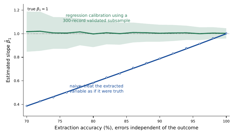
Figure 2:Extraction accuracy that sounds excellent produces estimates that are badly biased: at accuracy the naive slope recovers only about of the true effect, while regression calibration using a 300-record validated subsample is approximately unbiased across the whole range at the cost of wider intervals. Points are Monte Carlo means over 300 replicates (, , ); the blue line is the closed form the equation; the band is Monte Carlo standard deviation of the corrected estimator. :width: 90%
The derivation is short, and doing it is what makes the formula believable. The naive slope from regressing on is
Take the numerator first. Under non-differentiality, , so conditioning on and using the law of total covariance,
where the first term vanishes because and are conditionally independent given . Now and , so . Since covariance is unaffected by additive constants and scales linearly,
For the denominator, is Bernoulli with mean , so . Dividing, and using the identity (expand to check it), so that ,
which is the equation. The attenuation factor lies in whenever the extractor is better than a coin, equals one exactly when , and equals zero when , i.e. when carries no information about . The slope is pulled toward zero; the effect is diluted, never exaggerated.
That conclusion depends entirely on the term that vanished in the equation, and it is worth breaking the assumption on purpose, because an LLM is unusually well placed to break it. The vanishing term was , zero only because the extraction error was assumed independent of the outcome given the truth. A model reading a whole clinical note does not see in isolation; it sees the entire narrative, including language that predicts the outcome directly --- symptom descriptions, the tone of the assessment, incidental mentions of severity. If any of that language also nudges the extracted value , then and are no longer conditionally independent given , the first term in the equation is nonzero, and it adds to the numerator with a sign that need not be negative. This is differential misclassification, and its bias can go in either direction and can push the naive estimate past the truth. The simulation below sets both cases with the same true slope : the non-differential extractor attenuates as the formula predicts, while a differential extractor whose error rate also depends on inflates the estimate above .
import numpy as np

rng = np.random.default_rng(0)
n = 200000
pi, b0, b1 = 0.4, 0.0, 1.0
X = (rng.random(n) < pi).astype(float)
Y = b0 + b1 * X + rng.normal(0, 1.0, n)

def slope(y, x):                       # OLS slope of y on x
    x = x.astype(float)
    return np.cov(y, x, ddof=0)[0, 1] / np.var(x)

# Non-differential: X* depends on X only (se = sp = 0.85).
se, sp = 0.85, 0.85
flip = np.where(X == 1, rng.random(n) > se, rng.random(n) < 1 - sp)
Xstar_nd = np.where(flip, 1 - X, X)

# Differential: the extractor also reads outcome-related language, so the
# error rate depends on Y as well as X (a > 0 couples X* to Y given X).
a = 1.3
p_star = 1 / (1 + np.exp(-(-1.4 + 2.4 * X + a * Y)))
Xstar_d = (rng.random(n) < p_star).astype(float)

print(f"true beta1                              {b1:.3f}")
print(f"naive slope, non-differential error     {slope(Y, Xstar_nd):.3f}")
print(f"naive slope, differential error (a={a}) {slope(Y, Xstar_d):.3f}")
true beta1 1.000
naive slope, non-differential error 0.689
naive slope, differential error (a=1.3) 1.247The non-differential case lands where the equation says it should, below the truth. The differential case overshoots, and no amount of data corrects it, because the bias is again in the estimand. This is the single most important warning in the section: the reassuring “errors only attenuate” result is a theorem about an assumption that whole-document LLM extraction is built to violate, so it cannot be invoked as a general defence of a naive analysis. The only reliable guard is a validation subsample that measures the error structure directly, which is where the correction methods below get their leverage.
Three corrections are worth knowing, in increasing order of effort and of fidelity. The simplest is regression calibration: on the validation subsample, estimate --- for a binary field this is just the positive and negative predictive values --- and substitute that expectation for in the main regression Carroll et al., 2006. It removes the first-order attenuation and needs nothing beyond a second regression, which is why it is the default first move; its limitation is that it corrects the mean relation and can leave residual bias when the outcome model is nonlinear. Next is multiple imputation of the true value: treat as missing on the unlabelled records, fit an imputation model on the validation sample, draw several completed datasets, fit the analysis in each, and combine by Rubin’s rules. This uses the outcome and covariates in the imputation, so it handles differential error that regression calibration cannot, at the cost of a correctly specified imputation model. The most complete is a full likelihood or two-phase analysis, which writes the joint model for and maximises the observed-data likelihood over both phases, using the validation records where is known and marginalising over where it is not Carroll et al., 2006. It is the efficient estimator when the model is right and the most work to set up.
The point estimate is the easy part of all three; the variance is where people come to grief. A corrected slope depends on quantities --- the calibration coefficients, the imputation model, the phase-two likelihood --- that were themselves estimated from the finite validation sample, and treating them as known understates the standard error, sometimes badly. Regression calibration’s naive standard error ignores the uncertainty in ; multiple imputation needs Rubin’s between-imputation variance to be added; the two-phase MLE needs the full information matrix over both phases. The defensible default, and the one that sidesteps the algebra, is a bootstrap over the whole two-phase design Efron, 1979: resample documents and the validation labels together, re-run the entire correction on each resample, and take the empirical spread of the corrected estimate. That propagates both sources of uncertainty automatically and is the version to reach for unless a closed-form variance has been checked against it.
0.1.3Validation is a design problem, not a QA step
The temptation is to label a convenience batch of records, quote an accuracy, and proceed. Two design refinements pay for themselves. First, stratify the validation sample: oversample records the model flagged positive, since sensitivity is estimated only from true positives and those are scarce when prevalence is low, then reweight. Second, measure the human ceiling by double-labelling a subset, because an extraction pipeline cannot be shown to exceed an accuracy that your gold standard itself does not attain. (Annotation platforms such as Label Studio or doccano exist to make double-labelling, adjudication and inter-rater statistics a routine part of the design rather than something reconstructed from a spreadsheet afterwards.) A useful supplementary tool is conformal prediction, which converts any confidence score into extraction sets with finite-sample coverage under exchangeability Springer-Verlag, 2005Angelopoulos & Bates, 2021 --- for a categorical field, the model returns a set of candidate values guaranteed to contain the truth of the time, and the singleton sets can be accepted automatically while the rest route to a human. The coverage guarantee is only as good as its one assumption, and that assumption is exactly the one this setting tends to break: exchangeability between the calibration documents and the documents seen in deployment. Records from a new hospital, a new calendar year, or a new report template are not exchangeable with the set on which the conformal thresholds were tuned, so the coverage silently degrades precisely when the distribution shifts --- which is precisely when you most want a reliable set. The consequence is that conformal calibration must be refreshed whenever the document source changes, and its guarantee should be read as conditional on a stable population. The uncertainty-quantification chapter develops the exchangeability requirement and the behaviour of these methods under distribution shift in full, and the reader should take the machinery from there rather than have it repeated here.
One more threat to a validation estimate is specific to pretrained models and easy to miss. If the documents you validate on were plausibly in the model’s pretraining corpus, the accuracy you measure is optimistic, because the model may be recalling a value it saw during training rather than extracting it from the text in front of it. This is the classic leakage problem Kaufman et al., 2012 --- information from outside the intended input contaminating the estimate --- with a new mechanism: the leak is through the model’s weights rather than through a feature or a fold. It is most acute for published literature, where whole papers, their abstracts, and often their data tables are in the training data, so an extractor tested on public abstracts can post an accuracy it will not reproduce on the unpublished notes you actually care about. The mechanism is nearly impossible to rule out, since the pretraining corpus is not disclosed and cannot be audited. The partial defences are to validate on documents that post-date the model’s training cut-off, to prefer institutional records that were never public, and to treat any accuracy measured on well-known public corpora as an upper bound rather than an estimate of field performance.
0.1.4Implementation: schema-constrained extraction
The practical mechanics are simple enough to show in a dozen lines. Define the target record as a typed schema, require the model to emit that schema, and let the parser --- not the prose --- decide whether an output is admissible. Constrained decoding removes parse failures entirely; it removes no factual errors at all. (The constraint is enforced in one of two mechanically different ways --- a grammar-constrained decoder such as outlines, or the GBNF grammars built into llama.cpp, masks off-schema tokens so an invalid record is unreachable, whereas a validate-and-retry wrapper such as instructor re-prompts until the parser is satisfied --- and the difference matters to a statistician, because retrying until acceptance discards the hard documents non-randomly and quietly changes the population your data frame describes.)
class ChartRecord(BaseModel): patient_age: Optional[int] = Field(None, ge=0, le=120) smoking_status: Literal[“never”, “former”, “current”, “unknown”] biopsy_performed: bool evidence_span: str # verbatim quote supporting the fields above
1Ask the model for JSON conforming to ChartRecord.model_json_schema(),
2then parse. A parse failure is a rejected record, not a silent NaN.
record = ChartRecord.model_validate_json(model_output)
The evidence_span field earns its place by changing the economics of validation. Requiring the model to return the verbatim quote it based each value on turns auditing a record from a search problem into a lookup: instead of reading the whole note to confirm the smoking status, a human reads one sentence and checks whether the label follows from it. That is an check where the alternative is , and in practice it lets a validator get through fifty records in the time it would otherwise take to check ten --- which directly lowers the cost of the validation subsample the whole section depends on. It also localises disagreement: when the label is wrong you can see immediately whether the model quoted the wrong passage or read the right one incorrectly. What the field does not do is guarantee correctness. The model can quote a sentence accurately and still assign the wrong label to it --- quoting “patient quit smoking in 2015” and coding current --- so the evidence span speeds the audit without removing it. It makes errors cheap to catch, not impossible to make.
Where several records, draws, or passages bear on the same target value, they have to be aggregated, and the natural move is to take repeated draws from the model and vote --- self-consistency. The section on reliable and reproducible outputs develops when this helps and by how much, and the reader should take the details from there. The one point that belongs here is a warning against reading the vote as if it came from independent raters. Repeated draws from a single model, even at nonzero temperature, are positively correlated: they share the same weights, the same prompt, and the same misconceptions, so a systematic error is reproduced in every draw rather than averaged away. Majority voting over correlated draws reduces variance far less than the independent-rater calculation would suggest, and it does nothing at all about bias, because a mistake the model makes confidently it makes in every draw. Treat a self-consistency vote as one reading with a variance estimate, not as a panel of experts.
2.1Tools in practice
The tooling for extraction splits cleanly along the pipeline of Figure the figure, and the split is worth internalising because each stage has its own error process. Document conversion decides what text the model ever sees; constrained decoding decides what shape the output can take; the serving layer decides whether the instrument is stable enough to re-run; and the annotation layer decides whether you can measure any of it. Two habits are worth adopting before any of these are installed. First, measure the cheap baseline: a rule-based or dictionary-based extractor built with spaCy, or its biomedical variants scispaCy and medspaCy, often recovers structured fields such as dates, dosages and identifiers at an accuracy the language model must then be shown to beat, and it is deterministic and free. Second, remember that none of these tools estimates sensitivity or specificity for you; that number comes only from the validation subsample, and it is the number the rest of this section runs on.
[GROBID] Document structuring. Converts scholarly PDFs into structured TEI XML with the header, sections, tables and parsed reference list delimited as separate elements. Fits: stage one of a meta-analysis or literature-scale extraction, before any model call. Watch: conversion errors are silent and correlate with layout, so older scans and two-column tables lose content that then simply never appears in the data frame.
[Docling / Marker] Document structuring. General-purpose layout-aware converters that turn PDFs, office documents and scans into markdown or JSON with tables and reading order preserved. Fits: the same stage for non-scholarly sources --- reports, forms, regulatory submissions. Watch: table reconstruction is the weakest part of every such converter, and a merged or transposed table produces plausible numbers rather than an obvious failure.
[Outlines / llama.cpp grammars] Constrained decoding. Restrict generation to a formal grammar or JSON schema so that off-schema tokens are never sampled. Fits: the extraction call itself, when every record must parse. Watch: a schema-valid record is not a correct record; constraining the output space raises the admission rate and can lower accuracy per admitted record, which is exactly what the example below measures.
[Pydantic / Instructor] Schema and validation. Declare the target record as a typed model and reject anything that fails validation;
instructoradds an automatic re-prompt on failure. Fits: the schema-validation stage, and the definition of the record itself. Watch: log every rejection and every retry, because an unlogged retry loop turns a parse failure into a silently substituted record.[vLLM] Local serving. Runs open-weight models over a document corpus with high batch throughput and supports schema-constrained output. Fits: extraction at corpus scale, and any setting where documents cannot leave the institution. Watch: throughput settings such as batch size alter floating-point reduction order, so the instrument is only as stable as the serving configuration you record alongside the weights.
[Label Studio / doccano] Annotation. Interfaces for human labelling, adjudication and inter-annotator agreement over text spans and categorical fields. Fits: phase two --- the validation subsample and the double-labelled ceiling estimate. Watch: showing annotators the model’s proposed answer speeds labelling and biases it towards agreement, which inflates measured accuracy; label a fraction blind and compare.
The claim in the callouts that constrained decoding trades a parse-failure rate for a wrong-answer rate is easy to state and easy to get wrong, so measure it. The following replays stored outputs from two runs over the same six documents, one free-form and one schema-constrained, and applies the same admission gate to both. Nothing here calls a model; the responses are fixtures so that the arithmetic is reproducible.
SMOKING = (“never”, “former”, “current”, “unknown”)
def admit(raw): “”“Schema gate: parse, check types and levels. None = rejected.”“” try: r = json.loads(raw) except json.JSONDecodeError: return None ok = (set(r) == {“age”, “smoking”, “biopsy”} and isinstance(r[“age”], int) and 0 <= r[“age”] <= 120 and r[“smoking”] in SMOKING and isinstance(r[“biopsy”], bool)) return r if ok else None
def rec(a, s, b): return json.dumps({“age”: a, “smoking”: s, “biopsy”: b})
gold = [(61, “former”, True), (47, “never”, False), (73, “current”, True), (55, “never”, True), (38, “unknown”, False), (29, “never”, False)]
3Two runs over the same six documents, replayed from stored responses.
free = [rec(61, “former”, True), rec(47, “never”, False),
‘"json\n{"age": 73, ...}\n"’, # fenced: no parse
rec(55, “never”, True), rec(38, “unknown”, False),
‘The note gives no age. {“smoking”: “never”}’] # prose: no parse
constrained = [rec(61, “former”, True), rec(47, “never”, False),
rec(73, “former”, True), # admissible, wrong
rec(55, “never”, True), rec(38, “unknown”, False),
rec(29, “never”, False)]
def audit(name, outs): keep = [admit(o) for o in outs] n_ok = sum(k is not None for k in keep) n_right = sum(k is not None and tuple(k.values()) == g for k, g in zip(keep, gold)) print(f"{name:12s} admitted {n_ok}/6 correct {n_right}" f" acc|admitted {n_right / n_ok:.2f}" f" per document {n_right / 6:.2f}")
audit(“free-form”, free) audit(“constrained”, constrained)
Read the last two columns against each other. Accuracy conditional on admission is the number a dashboard will show you, and it moves the wrong way: the free-form run looks perfect because every record it failed to parse was silently dropped from the denominator. Accuracy per document is the estimand your downstream analysis actually needs, because a dropped record is a missing value, not an absence of error --- and it is missing precisely on the documents the model found hardest. The general lesson is the one this section keeps making: report the denominator you started with, not the one that survived.
3.1Exercises
Derive the equation from under non-differential misclassification. Verify when and when the extracted variable is independent of the truth.
With , compute the attenuation factor for , and . Explain why, at low prevalence, specificity matters far more than sensitivity for the bias in .
Construct an explicit differential-misclassification example in which the naive estimate is biased away from the null, and describe the feature of an LLM reading a full clinical note that makes this scenario realistic rather than contrived.
You will label records for validation. Write the expression for the standard error of and find the needed for a margin at . Then explain how stratifying on the model’s own prediction reduces that cost.
(Computational) Simulate the setting of Figure the figure: generate , corrupt it to at a chosen accuracy, and compare the naive slope, the closed form the equation, and a regression-calibration estimate using a validated subsample. Report bias, Monte Carlo standard deviation, and coverage of the nominal interval for each.
(Computational) Build a small extraction pipeline over 200 public abstracts using a schema of three fields. Hand-label a random 50, estimate per-field sensitivity and specificity with Wilson intervals Wilson, 1927, and report how the estimated effect of one extracted field on another changes before and after correction.
(Computational) Take the model’s per-field confidence scores, assess their calibration with a reliability diagram, and construct a route-to-human rule that attains precision on the auto-accepted subset. Report the fraction of records requiring human review, and check whether the routed records differ systematically from the rest.
- Guo, C., Pleiss, G., Sun, Y., & Weinberger, K. Q. (2017). On Calibration of Modern Neural Networks. Proceedings of the 34th International Conference on Machine Learning (ICML), 1321–1330.
- Carroll, R. J., Ruppert, D., Stefanski, L. A., & Crainiceanu, C. M. (2006). Measurement Error in Nonlinear Models. Chapman. 10.1201/9781420010138
- Efron, B. (1979). Bootstrap Methods: Another Look at the Jackknife. The Annals of Statistics, 7(1). 10.1214/aos/1176344552
- Algorithmic Learning in a Random World. (2005). Springer-Verlag. 10.1007/b106715
- Angelopoulos, A. N., & Bates, S. (2021). A Gentle Introduction to Conformal Prediction and Distribution-Free Uncertainty Quantification.
- Kaufman, S., Rosset, S., Perlich, C., & Stitelman, O. (2012). Leakage in Data Mining: Formulation, Detection, and Avoidance. ACM Transactions on Knowledge Discovery from Data, 6(4), 1–21. 10.1145/2382577.2382580
- Wilson, E. B. (1927). Probable Inference, the Law of Succession, and Statistical Inference. Journal of the American Statistical Association, 22(158), 209–212. 10.1080/01621459.1927.10502953