1AI for Scientific Writing
Scientific writing is the one place where a statistician’s professional reputation is transmitted in prose rather than in numbers, and it is also the task at which large language models are most obviously, and most dangerously, competent. A model trained to predict the next token has, in effect, been fit to the empirical distribution of published academic English; sampling from it produces text that reads exactly like the literature because that is what it was fit to Radford et al., 2019Brown et al., 2020. What it does not produce is a guarantee that any particular sentence is true, and a sentence that is fluent, on-topic, correctly formatted and false is a far more expensive error than one that is obviously garbled. The right posture for a statistician is therefore neither refusal nor delegation but measurement: treat the model as a fast, cheap, biased instrument, and treat your own reading of its output as a sampling-based audit whose power you can compute. This section develops that posture. We cover where the model genuinely helps --- second drafts, restructuring, reviewer responses, translating a methods section for a clinical audience --- where it reliably fails, how to design a verification protocol whose error rate you can state, and what the norms of authorship and disclosure currently demand.
Table 1:A dictionary for AI-assisted writing: nearly every failure mode of a language model in a manuscript has an established name in survey methodology, measurement, or quality control.
| ML / AI term | Statistical analogue | What is the same | What is different / the catch |
|---|---|---|---|
| Hallucination | Fabricated observation; measurement error with nonzero mean | Both report values that were never observed, biasing everything downstream | A fabricated citation is plausible by construction, so it survives the eyeball checks that catch data-entry error |
| Verification pass | Acceptance sampling of a finite lot | Inspect of items, infer the rest; the same operating characteristic | The defect rate is unknown and topic-dependent, and one missed defect can be disqualifying rather than merely costly |
| Retrieval augmentation | Conditioning on covariates rather than integrating over them | Both narrow the predictive distribution using supplied data | Retrieval supplies text, not truth; a retrieved passage constrains wording without validating the claim Lewis et al., 2020 |
| Sampling temperature | Tempered likelihood, | Low concentrates on the mode, high flattens | No makes the model accurate: temperature moves variance, not bias |
| Prompt / system instruction | Analysis protocol; the conditioning event in | Both fix the question before the answer is produced | Prompts are not identifiable from the output, so an unlogged prompt is an unlogged analysis choice |
| Style transfer to journal voice | Shrinkage toward the corpus mean | Both pull an idiosyncratic draft toward a population average | The target is the average paper; distinctive argument is exactly the signal that gets shrunk away |
| Perplexity of a passage | Held-out negative log-likelihood per observation | Identical formula, | Low perplexity means typical, not correct: a fit statistic, not a quality score |
| “AI-detector” output | A diagnostic test with sensitivity and specificity | Bayes’ rule applies; predictive value depends on prevalence | At realistic prevalence most positives are false, and non-native English writing is flagged at a higher rate |
| Automated literature screening | Two-stage screening in a systematic review | Both trade sensitivity for cost at stage one | Screening errors are not missing at random: what is under-represented in training, often the newest work, is dropped |
| Chain-of-thought trace | Showing the derivation beside the answer | Both make an argument auditable step by step | The trace is generated text, not a log of the computation that produced the answer Wei et al., 2022 |
| Disclosure statement | Methods section; data-provenance documentation | Both let a reader reconstruct what was done | Policy is in flux and version identifiers drift Mitchell et al., 2019Gebru et al., 2021 |
1.1What the model is actually good at
The useful cases share a structure: the ground truth is already in the author’s possession, and the model is asked only to re-express it. Tightening a paragraph you wrote, converting a bulleted outline into prose, generating three candidate titles, producing a plain-language abstract from a technical one, drafting a point-by-point reviewer response from your own notes, and translating a methods paragraph between an ML and a biostatistical register are all tasks where every factual claim originates with you and the model supplies only syntax. The failure cases share the complementary structure: the model is asked to supply content it does not have, most conspicuously references, effect sizes, and statements about what a particular cited paper found.
The distinction is mechanical enough to automate a first pass at it. Below, the same claim is put through “tighten this” and “write a paragraph about this”, and each output is scanned for assertions that cannot be traced back to the author.
import re

author_facts = {"n": "312", "hr": "0.78", "ci": "0.61-0.99", "level": "95"}
tightened = ("Among the 312 enrolled adults, the adjusted hazard ratio was "
             "0.78 (95% CI 0.61-0.99).")
generated = ("Among the 300 enrolled adults, the adjusted hazard ratio was "
             "0.80 (95% CI 0.65-0.98), consistent with Smith et al. (2019).")

def audit(text):
    nums = re.findall(r"\d+\.?\d*(?:-\d+\.?\d*)?", text)
    cites = re.findall(r"[A-Z][a-z]+ et al\. \(\d{4}\)", text)
    known = set(author_facts.values()) | {c[-5:-1] for c in cites}
    return nums, cites, [x for x in nums if x not in known]

for name, txt in [("tighten this", tightened),
                  ("write a paragraph", generated)]:
    nums, cites, unsupported = audit(txt)
    print(f"{name:<18} numbers={len(nums)}  citations={len(cites)}")
    print(f"{'':18} unverifiable numbers: {unsupported}")
    print(f"{'':18} citations to check:   {cites}")
print("\nask of every sentence: where did this fact come from?")
tighten this numbers=4 citations=0
unverifiable numbers: []
citations to check: []
write a paragraph numbers=5 citations=1
unverifiable numbers: ['300', '0.80', '0.65-0.98']
citations to check: ['Smith et al. (2019)']
ask of every sentence: where did this fact come from?The tightened version contains no fact the author did not supply, so it needs proofreading but not verification. The generated version contains four assertions with no provenance, three of which are wrong and one of which is a citation that may not exist. The audit burden is a property of the request, not of the model. It is at its worst for deep-research output, whose report format attaches a reference to every sentence and thereby maximises the number of claims requiring a check (Section that section).
The worked pair above is the whole diagnostic in miniature, and it is worth stating the rule it embodies explicitly, because it is the single habit that keeps AI-assisted writing honest. Ask of every sentence in a generated draft: where did this fact come from? If the answer is “from a table I made”, “from my own notes”, or “it is a rewording of something I wrote”, the sentence is safe and needs only proofreading. If the answer is “from the model”, the sentence is unverified, and it stays unverified until you trace the claim to a source that is not the model. The “tighten this” request produces text whose every fact answers the question with the author’s own input; the “write a paragraph about X” request produces text that answers it with the model, and therefore requires verification of every sentence. The point to internalise is that safety is not a property of the model or even of the topic --- it is a property of the request, and specifically of whether the request asked the model to re-express facts you already hold or to supply facts you do not.
This kind of on-command rewriting is recent enough to be worth a pointer to why it works. Instruction-tuned models Ouyang et al., 2022 are what made a request such as “rewrite this in the style of a methods section” succeed as a bare instruction; before instruction tuning you had to coax the same behaviour out of a base model by few-shot prompting, supplying worked examples of the transformation you wanted Brown et al., 2020. And the reason a single model can tighten, translate, summarise and restyle --- rather than needing a separate system for each --- is the text-to-text framing Raffel et al., 2020, which casts every such task as mapping an input string to an output string and so unifies them under one predictive model.
1.2Verification as an audit sample
Suppose a draft section contains checkable factual claims --- a citation that must say what you claim it says, a number that must match a table, a definition that must match the literature --- of which an unknown are wrong. You verify a simple random subset of of them. The number of errors you find is hypergeometric, so the probability that you catch at least one is
which is the operating characteristic of an acceptance-sampling plan. Two consequences are worth stating to any collaborator who proposes to “skim it for mistakes”. First, detection power is governed by , not by : a fixed number of errors is equally hard to find in a short section and a long one, so longer AI-assisted drafts are proportionally less safe at fixed reading effort. Second, finding no errors in a small sample is very weak evidence. Setting the right-hand side of the equation to and solving for gives the reading budget required for a stated detection guarantee; with claims, catching at least one of a mere two errors with probability 0.9 requires verifying 27 of them, which is most of the section. One stratum escapes this arithmetic entirely: a reference manager that resolves every DOI and arXiv identifier is a census rather than a sample, so the fabrication count it returns is exact and costs nothing.
Equation the equation is easier to believe once it is tabulated. The following evaluates the operating characteristic for a section with checkable claims.
from scipy.stats import hypergeom

m = 40
print("  e   k for 50%   k for 90%   Pr(catch >=1 | k=10)")
for e in (1, 2, 4, 8):
    oc = [1 - hypergeom.pmf(0, m, e, k) for k in range(m + 1)]
    k50 = next(k for k, v in enumerate(oc) if v >= 0.5)
    k90 = next(k for k, v in enumerate(oc) if v >= 0.9)
    print(f"{e:3d}   {k50:9d}   {k90:9d}   {oc[10]:.3f}")

print("\ndetection is governed by e, not by e/m:")
for m2 in (20, 40, 200):
    k = next(k for k in range(m2 + 1) if 1 - hypergeom.pmf(0, m2, 2, k) >= 0.9)
    print(f"  m={m2:3d} claims, e=2 errors -> verify {k:3d} "
          f"({100 * k / m2:4.1f}% of the section)")
e k for 50% k for 90% Pr(catch >=1 | k=10)
1 21 36 0.250
2 12 27 0.442
4 7 17 0.700
8 4 10 0.924
detection is governed by e, not by e/m:
m= 20 claims, e=2 errors -> verify 14 (70.0% of the section)
m= 40 claims, e=2 errors -> verify 27 (67.5% of the section)
m=200 claims, e=2 errors -> verify 137 (68.5% of the section)Two errors in forty claims require reading 27 of them for a chance of catching one, and reading ten gives you a coin-flip’s worth of assurance (0.442). The second block makes the fixed- point concrete: the required is roughly a constant fraction only because was held fixed while grew --- in a longer draft the same reading effort covers proportionally less, and the error count typically grows with the text.
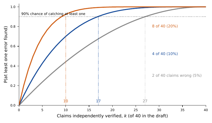
Figure 1:Spot-checking is much weaker than it feels: with 40 checkable claims in a section, catching at least one of two planted errors with probability 0.9 requires independently verifying 27 of them, and even a error rate demands 10. Curves are the hypergeometric operating characteristic the equation; dotted verticals mark the reading budget for detection. :width: 90%
The operational rule that follows is uncomfortable for the usual sales pitch. Because detection power is governed by the absolute error count , and because grows with the amount of text the model produced, verification cost scales with the volume of generation. The apparent economy of asking a model to draft a long passage is therefore mostly an illusion: the minutes saved in typing are paid back, often with interest, in the reading required to audit what was typed, and the longer the passage the worse the exchange rate. Priced honestly --- generation time plus audit time --- the case for using a model to produce substantive content is far weaker than the case for using it to reshape content you already have. There is one honest exception, and it is exactly what makes the good use cases good: text with no checkable claims carries no audit burden at all. A transition sentence, a topic sentence, a smoother phrasing of a point you already verified, a plain-language rewording of your own technical prose --- none of these asserts a fact that could be wrong, so by construction and the reading budget is zero. The economic case for AI drafting is strong precisely where the output contains nothing to verify, and it weakens in direct proportion to how many checkable claims the model was asked to manufacture.
The exchangeability assumption behind the equation is false in a way you can exploit: citations fail far more often than definitions do. Stratifying the audit by claim type dominates simple random sampling at equal cost.
from scipy.stats import hypergeom

strata = {"citations": (12, 0.25), "numbers": (18, 0.10),
          "definitions": (30, 0.02)}
m = sum(n for n, _ in strata.values())
e = sum(round(n * r) for n, r in strata.values())
k_srs = next(k for k in range(m + 1) if 1 - hypergeom.pmf(0, m, e, k) >= 0.90)
print(f"{m} claims, {e} expected errors, concentrated in citations")
print(f"simple random audit for 90% detection: read {k_srs} claims, "
      f"expected misses {e * (1 - k_srs / m):.2f}")

for plan in ({"citations": 12, "numbers": 18, "definitions": 5},
             {"citations": 12, "numbers": 7, "definitions": 0}):
    missed = sum(round(n * r) * (1 - plan[s] / n)
                 for s, (n, r) in strata.items())
    print(f"stratified plan {plan}")
    print(f"  read {sum(plan.values())} claims, expected misses {missed:.2f}")
60 claims, 6 expected errors, concentrated in citations
simple random audit for 90% detection: read 19 claims, expected misses 4.10
stratified plan {'citations': 12, 'numbers': 18, 'definitions': 5}
read 35 claims, expected misses 0.83
stratified plan {'citations': 12, 'numbers': 7, 'definitions': 0}
read 19 claims, expected misses 2.22The last plan reads the same 19 claims as the simple random audit and misses half as many errors, because it spends the budget where the defect rate is. The operational rule is short: verify every citation and every number, and sample the definitions.
Turned into a decision rule, the equation tells an author how much to read. Fix the tolerable error count --- the number of undetected errors you are willing to risk --- and the target detection probability , then solve for the smallest with . Table the table tabulates that for section lengths and error counts an author actually faces, and the numbers are sobering: except when errors are relatively plentiful, a genuine detection guarantee requires reading most of the section, which is the quantitative form of the claim that spot-checking does not certify a draft.
Table 2:Reading budget : the number of a section’s checkable claims that must be independently verified to detect at least one of errors with probability , from the equation. Except when errors are plentiful, the budget is most of the section.
| 20 | 0.90 | 18 | 14 | 9 |
| 20 | 0.95 | 19 | 16 | 10 |
| 40 | 0.90 | 36 | 27 | 17 |
| 40 | 0.95 | 38 | 31 | 21 |
| 80 | 0.90 | 72 | 55 | 35 |
| 80 | 0.95 | 76 | 62 | 42 |
The table assumes claims are exchangeable, and they are not: a citation is far more likely to be wrong than a definition, and a number transcribed from a table sits somewhere in between. That heterogeneity is not a nuisance but an opportunity, because a stratified audit that spends the reading budget where the defect rate is highest dominates simple random sampling at equal cost --- exactly as the toy example above shows, where a plan that reads the same number of claims misses half as many errors by concentrating on the citations. The operational recommendation is therefore not a single but a stratified rule: verify every citation and every number, since these are cheap to check and carry almost all the risk, and sample the definitions and other low-risk claims according to Table the table. Verifying every citation is especially affordable because, as the next tool section shows, existence is a census rather than a sample --- the identifiers either resolve or they do not.
1.3Why an “AI detector” is a diagnostic test, and a bad one
Journals and instructors increasingly run submissions through classifiers that claim to identify machine-generated text. Whatever the classifier’s internals, its output is a diagnostic test and Bayes’ rule applies:
with the prevalence of AI-written text in the submission stream. At , sensitivity 0.9 and specificity 0.9, the positive predictive value is exactly 0.5: a coin flip, applied to an accusation of misconduct. The error is also structured rather than random, because the classifiers key on low-perplexity, low-burstiness prose --- which is what careful non-native English writing looks like; detectors have been shown to flag non-native writers at sharply elevated rates Liang et al., 2023.
Working the equation numerically makes the position hard to argue with. The table uses an optimistic detector --- sensitivity and specificity both 0.95, better than published evaluations support.
sens, spec = 0.95, 0.95
print(" prevalence   PPV     NPV    false accusations per 100 flagged")
for pi in (0.02, 0.05, 0.10, 0.20, 0.50, 0.80):
    ppv = sens * pi / (sens * pi + (1 - spec) * (1 - pi))
    npv = spec * (1 - pi) / (spec * (1 - pi) + (1 - sens) * pi)
    print(f"   {pi:5.2f}     {ppv:.3f}   {npv:.3f}   {100 * (1 - ppv):5.1f}")

pi_star = (1 - spec) / (sens + 1 - spec)
print(f"\nPPV hits 0.5 at prevalence {pi_star:.3f}")
print(f"at sens=spec=0.90 the break-even prevalence is "
      f"{0.10 / (0.90 + 0.10):.3f}")
prevalence PPV NPV false accusations per 100 flagged
0.02 0.279 0.999 72.1
0.05 0.500 0.997 50.0
0.10 0.679 0.994 32.1
0.20 0.826 0.987 17.4
0.50 0.950 0.950 5.0
0.80 0.987 0.826 1.3
PPV hits 0.5 at prevalence 0.050
at sens=spec=0.90 the break-even prevalence is 0.100At a prevalence the positive predictive value is exactly 0.5, so half of the students or authors flagged are innocent, and at nearly three quarters are. A test with this operating characteristic can estimate a population rate; it cannot adjudicate an individual case, and using it that way is a misclassification error with a person attached to it.
The errors are also structured rather than random, which is the part that turns a measurement problem into a fairness problem. Detectors key on low perplexity and low burstiness, and careful non-native English writing has both.
import numpy as np
from statsmodels.stats.proportion import proportion_confint

rng = np.random.default_rng(0)
n = 400
# both groups wrote the text themselves; the second group's careful prose is
# lower-perplexity, which is what the detector actually keys on
flags = {"native": rng.random(n) < 0.05,
         "non-native": rng.random(n) < 0.19}
for name, f in flags.items():
    lo, hi = proportion_confint(f.sum(), n, method="wilson")
    print(f"{name:<11} flagged {f.mean():.3f}  95% CI ({lo:.3f}, {hi:.3f})")
rr = flags["non-native"].mean() / flags["native"].mean()
print(f"risk ratio {rr:.2f}: one group absorbs {rr:.1f}x the false positives")
print("specificity is not one number when the population is not homogeneous")
native flagged 0.045 95% CI (0.029, 0.070)
non-native flagged 0.168 95% CI (0.134, 0.207)
risk ratio 3.72: one group absorbs 3.7x the false positives
specificity is not one number when the population is not homogeneousBoth groups wrote every word themselves, and one absorbs nearly four times the false-positive rate. A single specificity figure quoted for a detector is a population average that conceals this; the quantity that matters for an accused author is the specificity in their subgroup, which is almost never reported.
The ethical reading of the equation is worth stating without hedging, because the numbers above leave little room for it. At a prevalence of the positive predictive value is 0.5; at it is about 0.83; only at an implausibly high does it reach 0.95 --- and these figures assume a detector far better than published evaluations support. A test with this operating characteristic can, in principle, estimate the population rate of AI-written text in a submission stream, provided its sensitivity and specificity have been validated on a labelled sample from that same stream. It cannot adjudicate an individual case: a positive result on one student’s essay or one author’s manuscript, at any realistic prevalence, is as likely to be wrong as right, and using it to support an accusation of misconduct attaches a person to a misclassification error. The problem is compounded by the structured nature of the errors --- non-native English writing is flagged at elevated rates --- so the false positives are not spread evenly across the population but concentrated on an identifiable group, which turns a measurement failure into a fairness failure. The chapter on the field’s ethical questions develops that fairness argument in full; here the narrow statistical conclusion suffices: a detector output is a diagnostic test, its individual predictive value is poor at realistic prevalence, and no institution should discipline a person on the strength of one.
1.4A provenance discipline for AI-assisted drafts
The reproducibility problem is the same one the field already solved for code and data: the output is a function of inputs that must be recorded. A minimally defensible workflow logs, for every generated passage, the model identifier and version, the full prompt including any system instruction, the decoding settings, the retrieved context if any, and the identity of the human who verified each factual claim. Figure the figure draws the loop. This is neither burdensome nor novel; it is a lab notebook, and the argument for it is the argument in Pineau et al. (2021) applied to prose rather than experiments.
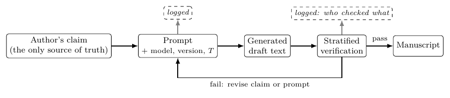
Figure 2:AI-assisted writing is reproducible only if the prompt, model version, decoding settings and per-claim verification record are logged; the model sits inside the loop as an instrument, never as a source of facts. :width: 90%
The record itself is small. A sidecar table with one row per checkable claim is enough to make a draft auditable, and it doubles as a submission checklist.
import hashlib
import pandas as pd

def h(s):
    return hashlib.sha256(s.encode()).hexdigest()[:10]

log = pd.DataFrame([
    {"claim_id": "c01", "kind": "number",
     "prompt_hash": h("draft results para v3"), "model": "assistant-2025-03",
     "temperature": 0.2, "verified_by": "KR", "source": "table2.csv"},
    {"claim_id": "c02", "kind": "citation",
     "prompt_hash": h("draft results para v3"), "model": "assistant-2025-03",
     "temperature": 0.2, "verified_by": "", "source": ""},
    {"claim_id": "c03", "kind": "definition",
     "prompt_hash": h("draft methods para v1"), "model": "assistant-2025-03",
     "temperature": 0.2, "verified_by": "BC", "source": "textbook"},
])
cols = ["claim_id", "kind", "prompt_hash", "verified_by", "source"]
print(log[cols].to_string(index=False))
open_items = log.query("verified_by == ''")
print(f"\nunverified claims blocking submission: "
      f"{list(open_items['claim_id'])}")
print(f"distinct prompts behind this section: {log['prompt_hash'].nunique()}")
claim_id kind prompt_hash verified_by source
c01 number 8f4820087d KR table2.csv
c02 citation 8f4820087d
c03 definition 0671db02e5 BC textbook
unverified claims blocking submission: ['c02']
distinct prompts behind this section: 2The value is in the last two lines: the log names the claim that nobody has checked, and it tells you how many distinct prompts stand behind the section, so a reader who wants to reproduce the draft knows what to ask for. Note the one-to-many structure --- a single prompt hash covers several claims, which is exactly why the prompt alone is not a sufficient record.
The record can be as light as a single sidecar file with one row per checkable claim, carried alongside the manuscript source in version control. The minimal column set is claim_id (a stable key you can cite in a comment in the draft), prompt_hash (a hash of the exact prompt and system instruction, so identical prompts collapse to one identifier and the prompt text can be stored once), model (the model identifier and version string the response reported), verified_by (the initials of the human who checked the claim, blank until someone has), and source (where the verified fact actually came from --- a table, a resolved DOI, a textbook). The toy example above emits exactly this table and derives the two facts that make it worth keeping: which claims remain unverified, and how many distinct prompts stand behind the section. A CSV is enough; a YAML block per claim is equivalent if you prefer to keep the prompt text inline. The one design point worth respecting is the one-to-many structure --- a single prompt produces several claims --- which is precisely why archiving the prompt alone is not a sufficient record and a per-claim row is.
What journal policy requires on top of this is still moving, but the settled points are two. First, disclosure: essentially every major venue now expects the use of AI tools to be stated, usually in the methods or the acknowledgements, with enough detail that a reader knows what was generated and how it was checked --- which is exactly what the sidecar documents. Second, and uniformly, a language model may not be listed as an author. The reason is not stylistic but definitional: authorship entails taking responsibility for the work, including its errors, and a model cannot be held responsible, so the accountability for every sentence remains entirely with the human authors regardless of who or what typed it. Consult the specific venue’s current instructions for the disclosure wording, since the format differs and changes; the underlying principle --- disclose the tool, never credit it as an author --- is stable.
LLM-assisted title and abstract screening is a two-stage design, and it should be reported as one: the model is stage one with an unknown sensitivity, and a human is stage two. The quantity to estimate before trusting it is the stage-one sensitivity, which requires a double-screened subsample.
import numpy as np
from statsmodels.stats.proportion import proportion_confint

rng = np.random.default_rng(0)
N, prev = 4000, 0.05
include = rng.random(N) < prev
sens, spec = 0.92, 0.70              # stage-one LLM screener
keep = np.where(include, rng.random(N) < sens, rng.random(N) < 1 - spec)
print(f"{N} records, {include.sum()} truly includable -> {keep.sum()} sent to "
      f"humans ({keep.mean():.0%} of the corpus)")
print(f"eligible studies dropped at stage one: {(include & ~keep).sum()}")

for nv in (300, 1000, 3000):
    v = rng.choice(N, nv, replace=False)   # double-screened subsample
    k, nn = (keep[v] & include[v]).sum(), include[v].sum()
    lo, hi = proportion_confint(k, nn, method="wilson")
    print(f"validation n={nv:4d}: sensitivity {k:3d}/{nn:3d} = {k / nn:.2f}  "
          f"95% CI ({lo:.2f}, {hi:.2f})")
4000 records, 212 truly includable -> 1313 sent to humans (33% of the corpus)
eligible studies dropped at stage one: 12
validation n= 300: sensitivity 14/ 14 = 1.00 95% CI (0.78, 1.00)
validation n=1000: sensitivity 45/ 48 = 0.94 95% CI (0.83, 0.98)
validation n=3000: sensitivity 141/150 = 0.94 95% CI (0.89, 0.97)The screener cuts the human reading burden to a third of the corpus at the cost of twelve eligible studies lost --- and the top validation row shows why the subsample must be large. Three hundred double-screened records contained only fourteen eligible studies, all of which the screener caught, giving an estimate of 1.00 with a lower bound of 0.78: perfectly compatible with the 0.92 sensitivity that is really there. Validation precision is governed by the number of eligible studies in the subsample, not by its size. (Open-source screeners such as ASReview implement this stage as an active-learning ranking with an explicit stopping rule Schoot et al., 2021, which makes the design auditable but does not supply the sensitivity estimate --- that still requires the double-screened subsample.)
The use case a statistician is most likely to meet first is systematic-review screening, and it is worth framing precisely because it is a two-stage design of a kind the reader already knows. In stage one, a model reads every title and abstract in a large candidate pool and predicts which are eligible; in stage two, a human reads only the records the model passed through. This is exactly a diagnostic screen with a human confirmatory stage, and its two operating characteristics have the usual meaning: the model’s sensitivity is the fraction of truly eligible studies it forwards, and its specificity is the fraction of ineligible ones it filters out. The economics are attractive --- the human reads a fraction of the corpus --- but the cost is measured in eligible studies lost at stage one, and a review that misses eligible studies is biased in a way no downstream analysis repairs. Text-mining and machine-learning approaches to this screening problem have a substantial literature O'Mara-Eves et al., 2015Marshall & Wallace, 2019, and the toy example above shows the design in action. The non-negotiable requirement is a validation subsample that is double-screened --- read by both the model and a human --- from which the model’s stage-one sensitivity is estimated before the pipeline is trusted, because, as the example makes plain, the precision of that estimate is governed by the number of eligible studies in the subsample rather than by its raw size, and eligible studies are scarce at realistic prevalence. Never inherit a sensitivity figure from a published evaluation on a different corpus; estimate it on yours.
1.5Writing quality is not a scalar, and automatic metrics know it
Machine-translation and summarisation research spent two decades learning that -gram overlap metrics such as BLEU Papineni et al., 2002 correlate only weakly with human judgement at the level of an individual document, even when they track system-level quality tolerably well. The statistical content of that lesson is that an automatic score is a surrogate endpoint: it is cheap, it is correlated with the thing you care about, and optimising it directly is how you destroy the correlation. If a model’s confidence in its own text is to be used at all, it should be scored with a proper scoring rule so that honest reporting is optimal Gneiting & Raftery, 2007, and it should be checked for calibration before it is believed, since neural models are systematically overconfident Guo et al., 2017.
The surrogate-endpoint argument is visible in two correlations computed from the same data. An automatic score can track quality well across systems while tracking it poorly within one, and optimising it directly breaks even that.
import numpy as np

rng = np.random.default_rng(0)
S, D = 10, 60                        # systems, documents each
sys_q = rng.normal(0, 0.7, S)
quality = sys_q[:, None] + rng.normal(0, 1.0, (S, D))
overlap = quality + rng.normal(0, 1.4, (S, D))   # a BLEU-like surrogate

doc_r = np.corrcoef(overlap.ravel(), quality.ravel())[0, 1]
sys_r = np.corrcoef(overlap.mean(1), quality.mean(1))[0, 1]
print(f"document-level corr(surrogate, quality) {doc_r:.3f}")
print(f"system-level   corr(surrogate, quality) {sys_r:.3f}")

gamed = overlap.copy()
gamed[3] += 1.5                      # system 3 optimises the surrogate only
print(f"best system: truth {int(np.argmax(quality.mean(1)))}, "
      f"surrogate {int(np.argmax(overlap.mean(1)))}, "
      f"surrogate after gaming {int(np.argmax(gamed.mean(1)))}")
rank3 = int(np.where(np.argsort(-quality.mean(1)) == 3)[0][0]) + 1
print(f"system 3 actually ranks {rank3} of {S} on true quality")
document-level corr(surrogate, quality) 0.649
system-level corr(surrogate, quality) 0.922
best system: truth 6, surrogate 6, surrogate after gaming 3
system 3 actually ranks 6 of 10 on true qualityThe system-level correlation of 0.92 is what a metrics paper reports; the document-level correlation of 0.65 is what you are relying on when you use the score to pick a draft. The last two lines are Goodhart’s law in three characters of code: one system raises its surrogate without touching its quality, and the metric now crowns a system that ranks sixth of ten on the thing you care about.
If a model’s own confidence is to be used as a triage signal --- verify the sentences it is least sure of --- it must first be checked for calibration against a proper scoring rule.
import numpy as np

rng = np.random.default_rng(0)
n = 4000
p = rng.uniform(0.5, 1.0, n)                     # the model's stated confidence
correct = rng.random(n) < np.clip(p - 0.18, 0, 1)  # accuracy lags it

edges = np.quantile(p, np.linspace(0, 1, 6))
idx = np.clip(np.digitize(p, edges[1:-1]), 0, 4)
print("stated conf    n     empirical accuracy    gap")
for b in range(5):
    m = idx == b
    acc = correct[m].mean()
    print(f"   {p[m].mean():.2f}      {m.sum():4d}          {acc:.3f}"
          f"          {acc - p[m].mean():+.3f}")
ece = sum((idx == b).mean() * abs(correct[idx == b].mean() - p[idx == b].mean())
          for b in range(5))
base = np.mean((correct.mean() - correct) ** 2)
print(f"\nECE {ece:.3f}   Brier {np.mean((p - correct) ** 2):.3f}   "
      f"Brier of the constant forecast {base:.3f}")
stated conf n empirical accuracy gap
0.55 800 0.362 -0.186
0.65 800 0.474 -0.176
0.75 800 0.589 -0.158
0.85 800 0.664 -0.185
0.95 800 0.769 -0.180
ECE 0.177 Brier 0.256 Brier of the constant forecast 0.245Every bin sits roughly 0.18 below its stated confidence, so the stated numbers are not probabilities and cannot be thresholded as such. The Brier score of 0.256 is worse than the constant forecast’s 0.245: this instrument’s confidences carry less information than ignoring them entirely. The ranking is still informative --- accuracy does increase across bins --- which is the useful distinction, since recalibration can fix a monotone miscalibration but cannot manufacture discrimination that is not there.
The general machinery for evaluating language-model outputs --- the design effects, the paired comparisons, the judge-model corrections --- belongs to the section on evaluating LLM outputs, and this section deliberately does not duplicate it. The one argument that had to appear here is the surrogate-endpoint argument, because it bears directly on the temptation to let an automatic score decide which draft is better: an automatic metric is a cheap proxy whose value rests entirely on its correlation with the quality you actually care about, that correlation is much weaker at the level of a single document than at the level of a system, and optimising the proxy directly is how you destroy the correlation. Take that as the reason not to hand the choice of wording to a metric, and take the fuller treatment from the evaluation section.
The standard this book endorses is simple and admits no exceptions. The author is responsible for every sentence in a manuscript, regardless of who or what produced the first draft of it. A model can tighten your prose, translate your register, and propose a structure; it cannot assume responsibility for a claim, and so it cannot relieve you of the obligation to verify one. Every technique in this section --- the audit sample, the stratified verification, the provenance log, the refusal to treat a detector’s verdict as proof --- is an instrument in service of that single standard. Use the tools freely for what they are good at, price the verification honestly for what they are not, and never let the fluency of a generated sentence substitute for knowing that it is true.
1.6Tools in practice
Sorted by the criterion that runs through this section --- whether the tool supplies content or only syntax --- the writing tools split cleanly. Anything that rewrites text you wrote adds no checkable claims and needs proofreading only. Anything that supplies references, numbers or statements about what a paper found adds claims at a rate you must audit, and the audit is the expensive half of the workflow. A third group does neither: it verifies, and these are the ones that reduce the reading budget derived above rather than inflating it. Journal and publisher policies on disclosure are also in flux; consult the specific venue’s current instructions rather than any summary printed here.
[General-purpose chat assistants] Text transformation. Tighten, restructure, retitle, or convert a technical abstract to plain language. Fits: the safe half of this section --- every fact in the output came from your input. Watch: the boundary is crossed silently the moment you ask for content rather than form; the audit burden is set by the request, not the tool.
[Deep-research assistants] Multi-step search and synthesis with citations. Return a structured report whose sentences carry inline references. Fits: a starting bibliography and a map of a subfield. Watch: the report format transfers unearned authority to every sentence; Section that section treats the verification of such output as the measurement problem it is.
[Overleaf / Writefull / Grammarly] Manuscript-embedded language assistance. Suggest wording, grammar and register changes in place. Fits: the shrinkage-toward-the-corpus-mean use case, which is genuinely useful for a non-native writer facing a native-speaker reviewer. Watch: the same shrinkage flattens a deliberately unusual sentence, and accepting every suggestion is how a distinctive argument becomes an average paper.
[Zotero / Better BibTeX] Reference management with identifier resolution. Fetch metadata by DOI or arXiv identifier and emit a canonical entry. Fits: the mechanical half of citation checking --- an entry that will not resolve is a fabrication, detected at zero marginal cost. Watch: resolution certifies existence and nothing else; whether the paper supports your sentence is a question only reading answers.
[ASReview] Active-learning screening. Reorders titles and abstracts by predicted relevance so that eligible studies are found early in the screening queue Schoot et al., 2021. Fits: stage one of the two-stage screening design measured above, with an explicit stopping rule. Watch: the ranking’s sensitivity is a property of your corpus and your inclusion criteria, so it must be estimated from a double-screened subsample and not inherited from a published evaluation.
[Quarto / R Markdown] Literate manuscripts. Compute the numbers in the document that reports them. Fits: eliminating an entire stratum from the audit --- a number written by code from the data cannot be a transcription error or a hallucination. Watch: it removes the numbers stratum only; citations and definitions are untouched, and by the stratified argument above they were the expensive ones anyway.
Reference managers make the mechanical check free, which sharpens rather than solves the problem: the check that costs nothing catches the error that matters least. The example below runs the resolution pass over a small bibliography containing one fabricated entry and one entry whose identifier resolves to a different paper, then prices what is left. The resolver here is a local dictionary so the example runs offline; the real version issues one request per identifier, as in
curl -s https://api.crossref.org/works/10.1038/s41598-023-41032-5
curl -s "http://export.arxiv.org/api/query?id_list=2104.11222"
and compares the returned title against the one in the entry.
# offline stand-in for Crossref / arXiv: the real version resolves each id
RECORDS = {
    "10.1038/s41598-023-41032-5":
        "Fabrication and errors in the bibliographic citations generated by "
        "ChatGPT",
    "10.1038/s42256-020-00287-7":
        "An open source machine learning framework for efficient and "
        "transparent systematic reviews",
    "2104.11222": "On Aliased Resizing and Surprising Subtleties in GAN "
                  "Evaluation",
}

def resolve(identifier):
    return RECORDS.get(identifier)

def norm(s):
    return " ".join(s.lower().replace("-", " ").split())

bib = [
    ("walters2023", "10.1038/s41598-023-41032-5",
     "Fabrication and errors in the bibliographic citations generated by "
     "ChatGPT"),
    ("vandeschoot2021", "10.1038/s42256-020-00287-7",
     "An open source machine learning framework for efficient and "
     "transparent systematic reviews"),
    ("parmar2022", "2104.11222",
     "On Aliased Resizing and Surprising Subtleties in GAN Evaluation"),
    ("ghost2021", "10.1038/s41586-021-99999-9",       # planted: no such record
     "Deep generative models for automated systematic review"),
    ("swapped2019", "10.1038/s42256-020-00287-7",     # real id, wrong title
     "Active learning reduces screening effort in clinical meta-analysis"),
]

for key, ident, claimed in bib:
    got = resolve(ident)
    if got is None:
        verdict = "UNRESOLVABLE -- likely fabricated"
    elif norm(got) == norm(claimed):
        verdict = "resolves, title matches"
    else:
        verdict = "RESOLVES TO A DIFFERENT WORK"
    print(f"{key:<16} {verdict}")

n = len(bib)
caught = sum(resolve(i) is None or norm(resolve(i)) != norm(t)
             for _, i, t in bib)
print(f"\nmechanical pass flagged {caught}/{n} entries")
print(f"entries it certified as existing: {n - caught}")
print(f"entries whose sentence it verified: 0 -- support still costs "
      f"{n - caught} reads")
walters2023 resolves, title matches
vandeschoot2021 resolves, title matches
parmar2022 resolves, title matches
ghost2021 UNRESOLVABLE -- likely fabricated
swapped2019 RESOLVES TO A DIFFERENT WORK
mechanical pass flagged 2/5 entries
entries it certified as existing: 3
entries whose sentence it verified: 0 -- support still costs 3 reads
mechanical pass flagged 2/5 entries
entries it certified as existing: 3
entries whose sentence it verified: 0 -- support still costs 3 readsTwo errors are caught for free, and they are two different errors: an identifier that resolves to nothing, and an identifier that resolves to a real paper other than the one claimed. Both are a census, not a sample --- every entry is checked, so the fabrication count is exact rather than estimated, and this is the one place in the audit where the hypergeometric arithmetic of the equation does not apply. What the pass cannot do is the last line. Three entries are certified to exist and none is certified to support the sentence it is attached to, so the reading budget is unchanged by the tool that appeared to solve the problem. Fabricated citations from chatbots have been measured directly and are common enough to take seriously Walters & Wilder, 2023, but a bibliography with a zero fabrication rate is not a verified bibliography --- it has passed the cheap test, and the expensive one is still ahead. Run the census on every entry, then spend the sampling budget from the stratified plan on whether the papers say what you claim they say.
1.7Exercises
Derive the equation from the hypergeometric distribution, and show that for fixed the required sample size to attain detection probability grows only slowly in . Interpret the consequence for long AI-assisted drafts.
A section contains checkable claims. You are willing to accept a chance of missing all errors if there are . How many claims must you verify? Repeat for and comment on whether spot-checking can ever certify a draft.
Using the equation, plot positive predictive value against prevalence for a detector with sensitivity 0.95 and specificity 0.95. State the prevalence below which a positive result is more likely false than true, and write two sentences on why this rules out the individual-adjudication use case.
(Computational) Take a paragraph you have written and ask a language model to (a) tighten it and (b) write a new paragraph on the same topic. Enumerate the checkable claims in each output, verify all of them, and record the error rate separately for the two conditions. Report the two counts and the time spent verifying.
(Computational) Ask a model for ten references on a topic you know well. For each, check existence, authorship, year and whether it supports the claim it was offered for. Classify errors as non-existent, real but misattributed, or real but irrelevant, and estimate each rate with a Wilson interval.
(Computational) Take the reference list of a draft and run the mechanical pass over it: resolve every DOI through Crossref and every arXiv identifier through the arXiv API, and compare the returned title with the one in your entry. Report the count of unresolvable entries, the count that resolve to a different work, and --- separately --- the number of entries whose support for the attached sentence remains unverified.
(Computational) Generate the same abstract at temperatures 0.2, 0.7 and 1.2, five draws each. Have a colleague rank all fifteen blind. Fit an ordinal model with temperature as the predictor and report whether the effect on rank is distinguishable from zero at this sample size --- then compute the number of draws that would be needed if it were not.
- Radford, A., Wu, J., Child, R., Luan, D., Amodei, D., & Sutskever, I. (2019). Language Models are Unsupervised Multitask Learners [Techreport]. OpenAI.
- Brown, T. B., Mann, B., Ryder, N., Subbiah, M., Kaplan, J., Dhariwal, P., Neelakantan, A., Shyam, P., Sastry, G., Askell, A., Agarwal, S., Herbert-Voss, A., Krueger, G., Henighan, T., Child, R., Ramesh, A., Ziegler, D. M., Wu, J., Winter, C., … Amodei, D. (2020). Language Models are Few-Shot Learners.
- Lewis, P., Perez, E., Piktus, A., Petroni, F., Karpukhin, V., Goyal, N., Küttler, H., Lewis, M., tau Wen-Yih, Rocktäschel, T., Riedel, S., & Kiela, D. (2020). Retrieval-Augmented Generation for Knowledge-Intensive NLP Tasks.
- Wei, J., Wang, X., Schuurmans, D., Bosma, M., Ichter, B., Xia, F., Chi, E., Le, Q., & Zhou, D. (2022). Chain-of-Thought Prompting Elicits Reasoning in Large Language Models.
- Mitchell, M., Wu, S., Zaldivar, A., Barnes, P., Vasserman, L., Hutchinson, B., Spitzer, E., Raji, I. D., & Gebru, T. (2019). Model Cards for Model Reporting.
- Gebru, T., Morgenstern, J., Vecchione, B., Vaughan, J. W., Wallach, H., III, H. D., & Crawford, K. (2021). Datasheets for Datasets.
- Ouyang, L., Wu, J., Jiang, X., Almeida, D., Wainwright, C. L., Mishkin, P., Zhang, C., Agarwal, S., Slama, K., Ray, A., Schulman, J., Hilton, J., Kelton, F., Miller, L., Simens, M., Askell, A., Welinder, P., Christiano, P., Leike, J., & Lowe, R. (2022). Training language models to follow instructions with human feedback.
- Raffel, C., Shazeer, N., Roberts, A., Lee, K., Narang, S., Matena, M., Zhou, Y., Li, W., & Liu, P. J. (2020). Exploring the Limits of Transfer Learning with a Unified Text-to-Text Transformer.
- Liang, W., Yuksekgonul, M., Mao, Y., Wu, E., & Zou, J. (2023). GPT detectors are biased against non-native English writers. Patterns, 4(7), 100779. 10.1016/j.patter.2023.100779
- Pineau, J., Vincent-Lamarre, P., Sinha, K., & others. (2021). Improving Reproducibility in Machine Learning Research.
- van de Schoot, R., de Bruin, J., Schram, R., Zahedi, P., de Boer, J., Weijdema, F., Kramer, B., Huijts, M., Hoogerwerf, M., Ferdinands, G., & others. (2021). An open source machine learning framework for efficient and transparent systematic reviews. Nature Machine Intelligence, 3(2), 125–133. 10.1038/s42256-020-00287-7
- O’Mara-Eves, A., Thomas, J., McNaught, J., Miwa, M., & Ananiadou, S. (2015). Using text mining for study identification in systematic reviews: a systematic review of current approaches. Systematic Reviews, 4(1), Article 5. 10.1186/2046-4053-4-5
- Marshall, I. J., & Wallace, B. C. (2019). Toward systematic review automation: a practical guide to using machine learning tools in research synthesis. Systematic Reviews, 8(1), Article 163. 10.1186/s13643-019-1074-9
- Papineni, K., Roukos, S., Ward, T., & Zhu, W.-J. (2002). BLEU: a Method for Automatic Evaluation of Machine Translation. Proceedings of the 40th Annual Meeting of the Association for Computational Linguistics (ACL), 311–318. 10.3115/1073083.1073135
- Gneiting, T., & Raftery, A. E. (2007). Strictly Proper Scoring Rules, Prediction, and Estimation. Journal of the American Statistical Association, 102(477), 359–378. 10.1198/016214506000001437