1AI Agents
An agent is a language model placed in a loop: it observes a state, chooses an action from a set of available tools, sees the result, and repeats until it decides it is finished. Nothing about the model changes --- it is the same conditional distribution over tokens as in the previous sections --- but the object of study does, because a single response is no longer the unit of analysis. What matters is the trajectory, and trajectories have properties that single responses do not: errors compound, the state the model conditions on is one it partly created, and the outcome is a function of choices made many steps earlier. This is a sequential decision problem, and statisticians will recognize most of its structure from reinforcement learning, sequential design, and the analysis of longitudinal data with time-varying treatment. This section develops that correspondence, gives the arithmetic of compounding failure that governs how long an agent can run before it becomes useless, and argues that evaluating an agent is a harder measurement problem than evaluating a model --- one that the field currently handles with sample sizes a statistician would reject on sight.
Table 1:Agentic vocabulary is largely reinforcement-learning and sequential-decision vocabulary with the training removed; the last column marks where that omission matters.
| ML / AI term | Statistical analogue | What is the same | What is different / the catch |
|---|---|---|---|
| Agent | A policy in a sequential decision problem | Maps observed state to an action | The policy is a frozen pretrained model prompted at run time, not one fitted to this task |
| Tool call / function calling | A structured query with a typed argument list | Constrained, validatable input | Arguments are generated text; validation is on you, and a malformed call can be silently retried |
| Trajectory / episode | A subject’s observation sequence in a longitudinal study | An ordered record of states and actions | Actions change the state, so later observations are not exchangeable with earlier ones |
| Reward / task success | The outcome variable | The thing being optimized or measured | Usually binary and end-of-episode, giving very little information per run |
| Planning | Sequential experimental design | Choosing the next action to reduce uncertainty | No explicit uncertainty model; the “plan” is generated text |
| ReAct (reason then act) | Interleaving analysis and data collection | Alternate between thinking and observing | The reasoning trace is not a faithful account of the computation and should not be read as one |
| Self-consistency / majority voting | Bagging; the bootstrap-aggregated vote | Average several stochastic runs | The runs share a model, so errors are correlated and the variance reduction is limited |
| Memory / scratchpad | A running sufficient statistic; a state vector | Carries information forward | Unbounded, unstructured text, so old mistakes persist and are re-conditioned on |
| Guardrail | A constraint on the action space | Rules out inadmissible actions | Enforced by prompt or by code; only the second kind is a real constraint |
| Human in the loop | Sequential monitoring with a stopping rule | A person approves or halts | The approval decision is itself error-prone and fatigues |
| Multi-agent system | An ensemble or a committee of experts | Multiple models combined | Communication is text, so errors propagate rather than average out |
| Compounding error | Error propagation in a multi-step forecast | Small per-step error accumulates | Geometric in trajectory length, so reliability targets are brutal |
| Agent benchmark | A small experiment with a binary endpoint | Estimating a success probability | Typically 30--200 episodes, so intervals are points or worse |
| Cost per task | Total variable cost of one experimental unit | Resource accounting | Highly skewed across episodes; report a median and a tail, never a mean alone |
1.1The Loop, Written Down
At step the agent conditions on a history of the task description, the actions it took, and the observations they returned, and samples an action from the model,
where is the environment --- a search index, a Python interpreter, a database, a filesystem. Interleaving a generated rationale with each action, as in ReAct Yao et al., 2022, is the pattern almost every framework now follows. This is exactly the policy-and-environment structure of reinforcement learning Sutton, 1988Mnih et al., 2015, with one decisive difference: was not fitted to this environment. It is a general-purpose text model being asked to behave like a policy, and the entire engineering discipline of “agent building” consists of shaping --- through instructions, tool descriptions, and what is kept in memory --- so that the sampled actions are sensible.
The loop is short enough to write out in full. The example below is a two-tool agent with a hard step limit; watch the history grow, and note that the only thing carrying information between steps is the text in \verb|h|.
import re

FACTS = {"n_patients": "312", "site_count": "4"}
TOOLS = {"calc": lambda a: str(eval(a, {"__builtins__": {}})),
         "lookup": lambda a: FACTS.get(a, "NOT_FOUND")}

def policy(task, h):          # stands in for a_t ~ pi_theta( . | h_t)
    seen = " ".join(h)
    for key in FACTS:
        if key in task and key not in seen:
            return ("lookup", key)
    nums = re.findall(r"\d+", seen)
    if len(nums) >= 2 and "calc" not in seen:
        return ("calc", f"{nums[0]}/{nums[1]}")
    return ("stop", "")

task = "average n_patients per site given site_count"
h, LIMIT = [], 6
for t in range(1, LIMIT + 1):
    a, arg = policy(task, h)
    if a == "stop":
        print(f"t={t}  |h_t|={len(h)}  action=stop")
        break
    o = TOOLS[a](arg)
    print(f"t={t}  |h_t|={len(h)}  action={a + '(' + arg + ')':<22} obs={o}")
    h.append(f"{a}({arg})->{o}")
else:
    print("hit the step limit without stopping")
print("history:", " | ".join(h))
t=1 |h_t|=0 action=lookup(n_patients) obs=312
t=2 |h_t|=1 action=lookup(site_count) obs=4
t=3 |h_t|=2 action=calc(312/4) obs=78.0
t=4 |h_t|=3 action=stop
history: lookup(n_patients)->312 | lookup(site_count)->4 | calc(312/4)->78.0Nothing here is learned. The “policy” is a fixed rule reading a text history, and the three tool calls are the whole trajectory --- which is exactly the point: the object being analysed is the sequence, not any one response. (Orchestration libraries such as LangGraph make the same loop explicit as a graph of nodes with checkpointed state, which is what allows a failed step to be retried without replaying the whole trajectory.)
Tool calling is constrained generation, and the constraint is enforced by a schema validator rather than by the model. The example asks what a retry budget buys when the raw call is malformed one time in three.
import json
import numpy as np

rng = np.random.default_rng(0)
SCHEMA = {"name": str, "args": dict}

def emit():                    # the model's raw tool call, sometimes malformed
    r = rng.random()
    if r < 0.20:
        return '{"name": "lookup", "args": {"key": "n"}'       # truncated
    if r < 0.30:
        return '{"name": "lookup", "arguments": {"key": "n"}}'  # bad field
    return '{"name": "lookup", "args": {"key": "n"}}'

def valid(s):
    try:
        c = json.loads(s)
    except json.JSONDecodeError:
        return False
    return all(k in c and isinstance(c[k], t) for k, t in SCHEMA.items())

raw = np.mean([valid(emit()) for _ in range(4000)])
print(f"validity of one raw call   {raw:.3f}")
for r in (2, 3, 4):
    ok = [any(valid(emit()) for _ in range(r)) for _ in range(4000)]
    print(f"valid within {r} attempts    {np.mean(ok):.3f}")
validity of one raw call 0.701
valid within 2 attempts 0.910
valid within 3 attempts 0.977
valid within 4 attempts 0.995Validation plus retries turns a 0.70 generator into a 0.98 one at three attempts, which is geometric decay of the failure probability and ordinary software engineering. It works only because a malformed call is cheap to detect; nothing here improves the semantic correctness of a call that parses. (Typed-output libraries such as Pydantic AI and Instructor package this exact loop, binding a call to a declared schema and re-prompting on a parse failure, which is why the reliability of an agent framework is usually a property of its validator rather than of its model.)
It is worth making the reinforcement-learning correspondence explicit and early, because it orients the structure and, more usefully, tells an RL-literate reader what is missing. Equation the equation is a policy acting in an environment and generating a trajectory --- the setup of Sutton (1988) and, in its modern deep form, Mnih et al. (2015). What is absent is everything that makes reinforcement learning learning: there is no value function estimating the return from a state, no credit assignment attributing the final outcome to the actions that caused it, and no training on the environment’s rewards. The agent is a policy with no policy-improvement step. It executes; it does not update. Every technique in this section is therefore an attempt to get good behaviour out of a fixed policy by shaping what it conditions on, not by improving the policy itself --- which is why prompt engineering, tool descriptions, and memory management do here the work that gradient steps do in reinforcement learning.
Tool calling deserves a second look as a statistical object, because it is where the agent touches the world and where most of the engineering effort goes. A tool call is constrained generation: the model emits text that must conform to a declared schema --- a function name and a typed argument list --- before it can be executed. That the model can produce such calls at all is not obvious, and it need not be prompted into existence. Schick et al. (2023) showed that tool use can be learned, with a model taught during training which interface to call and with what arguments, by self-supervision on whether the call improved its own next-token prediction. In deployment, though, the reliability of the whole system rarely rests on the model’s fluency with the schema. It rests on schema validation and retries --- ordinary software engineering, not machine learning. A validator parses the emitted call, rejects the malformed ones, and re-prompts; the arithmetic of that loop is the example above, and it is the same geometric decay of failure probability that any retry protocol enjoys. The lesson worth carrying is that the machine-learning content of tool use is small and the software-engineering content is large, and a team that treats it the other way around will spend its time tuning prompts when it should be writing a validator.
1.2Why Long Trajectories Fail
Suppose each step succeeds independently with probability and the task requires steps, all of which must be right. Then
so at a per-step reliability of 0.95 --- which sounds excellent --- a 20-step task succeeds barely a third of the time. This crude geometric model is the most useful single thing to know about agents, because it converts a vague complaint about unreliability into a design constraint: either raise , shorten , or introduce checkpoints that allow recovery so the failures stop being absorbing. Independence is of course wrong, and it is wrong in the unhelpful direction, since a bad early action corrupts the history that every later action conditions on, which induces positive dependence between failures.
The arithmetic is worth seeing rather than asserting. The table below evaluates the equation across per-step reliabilities that all sound acceptable, and then inverts it to give the reliability a target trajectory length demands.
import numpy as np

T = np.array([1, 5, 10, 20, 50])
print("        T =  " + "".join(f"{t:7d}" for t in T) + "   E[steps to fail]")
for p in (0.90, 0.95, 0.99):
    row = "".join(f"{p ** t:7.3f}" for t in T)
    print(f"p={p:.2f}  p^T {row}        {1/(1-p):7.1f}")
print()
for t in (10, 30, 100):
    print(f"a {t:3d}-step task at 90% overall needs p >= {0.9 ** (1/t):.4f}")
T = 1 5 10 20 50 E[steps to fail]
p=0.90 p^T 0.900 0.590 0.349 0.122 0.005 10.0
p=0.95 p^T 0.950 0.774 0.599 0.358 0.077 20.0
p=0.99 p^T 0.990 0.951 0.904 0.818 0.605 100.0
a 10-step task at 90% overall needs p >= 0.9895
a 30-step task at 90% overall needs p >= 0.9965
a 100-step task at 90% overall needs p >= 0.9989The inversion is the uncomfortable half: a 30-step task that succeeds nine times in ten requires per step. No prompt achieves that, which is why the practical response is to shorten rather than to chase .
Independence is the assumption that makes the equation tractable, and it fails in the unhelpful direction. Two mechanisms do the damage: reliability that decays as the history fills with the agent’s own output, and an episode-level difficulty shared by every step.
import numpy as np

T = 20
p_t = 0.97 * 0.985 ** np.arange(T)   # reliability decays as h_t grows
print(f"step-1  reliability {p_t[0]:.3f}   (what a short benchmark sees)")
print(f"step-{T} reliability {p_t[-1]:.3f}   (what the agent has by then)")
print(f"iid extrapolation p1^T {p_t[0] ** T:.3f}   "
      f"actual product {np.prod(p_t):.3f}")

rng = np.random.default_rng(0)
b = rng.normal(0.0, 0.8, 400000)       # episode effect, shared by all steps
p_ep = 1.0 / (1.0 + np.exp(-(1.9 + b)))
print(f"mean per-step reliability {p_ep.mean():.3f}")
print(f"iid extrapolation of that mean   {p_ep.mean() ** T:.3f}")
print(f"with the shared episode effect   {np.mean(p_ep ** T):.3f}")
step-1 reliability 0.970 (what a short benchmark sees)
step-20 reliability 0.728 (what the agent has by then)
iid extrapolation p1^T 0.544 actual product 0.031
mean per-step reliability 0.845
iid extrapolation of that mean 0.034
with the shared episode effect 0.125Both mechanisms make the geometric model optimistic when it is calibrated on step-one behaviour and pessimistic when it is calibrated on a marginal per-step rate: a random-effects structure puts mass on episodes that go perfectly and on episodes that fail immediately. Either way, a per-step success rate measured on short trajectories does not extrapolate to long ones.
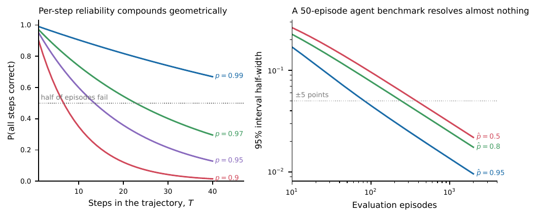
Figure 1:Two pieces of arithmetic that constrain what agents can do. Left: the equation, the probability that every step of a -step trajectory succeeds. Reliability that would be impressive in a single response is not enough to complete a long task, which is why practical systems shorten trajectories and add checkpoints rather than chasing a better prompt. Right: the half-width of a 95% Wilson interval for a success probability as a function of the number of evaluation episodes. At the 50 to 100 episodes typical of published agent benchmarks, the interval is roughly points, so most reported comparisons between agents are not resolvable. :width: 90%
The two panels together give the design brief. Because completion probability is and the interval on any measured success rate is wide, the winning move is almost never to chase a better prompt: it is to reduce and to make each step self-checking. Decompose a long task into short subtasks whose individual results can be verified --- ideally by code rather than by the model, since a check the model performs on itself shares the model’s blind spots --- and prefer an architecture in which a failed step is caught and retried locally rather than written into , where it becomes a premise every later step conditions on. A failure retried in place costs a few tokens; a failure that poisons the history costs the whole trajectory. This is the same instinct that leads a statistician to break a fragile long computation into checkpointed, independently validated stages rather than to run it end to end and inspect only the final number.
1.3Verification Is the Whole Game
The asymmetry that makes agents work at all is that many useful actions are far easier to check than to produce. A generated SQL query either parses and returns rows or does not; a script either runs the unit tests or fails them; a proposed citation either resolves to a real record or does not. Where a cheap, automatic verifier exists, an agent can afford to be wrong often, because it can sample, check, and retry --- and the failure probability falls geometrically in the number of independent attempts. Where no verifier exists --- summarizing a literature, interpreting a result, drafting a conclusion --- there is no such recovery, and the agent’s output must be treated as a draft requiring human adjudication. The deep-research agents of Section that section sit squarely in this second regime, and the sampling-based verification developed there is what replaces the missing verifier. This distinction, rather than any property of the model, is the best available predictor of whether an agentic workflow will succeed in a given scientific task.
Checkpoints change the arithmetic because they make a failure recoverable rather than absorbing. Suppose a failed step is caught by a verifier with detection probability and retried up to times; the effective per-step success rate becomes with .
p, T = 0.85, 20
q = 1 - p
print("detect  k=1     k=3     k=10    ceiling  Pr(20 steps | k=3)")
for d in (1.0, 0.9, 0.5, 0.0):
    eff = [p * (1 - (q * d) ** k) / (1 - q * d) for k in (1, 3, 10)]
    ceiling = p / (p + q * (1 - d))
    print(f"{d:5.2f}  " + "  ".join(f"{e:.4f}" for e in eff)
          + f"  {ceiling:.4f}   {eff[1] ** T:.4f}")
detect k=1 k=3 k=10 ceiling Pr(20 steps | k=3)
1.00 0.8500 0.9966 1.0000 1.0000 0.9346
0.90 0.8500 0.9802 0.9827 0.9827 0.6709
0.50 0.8500 0.9185 0.9189 0.9189 0.1828
0.00 0.8500 0.8500 0.8500 0.8500 0.0388The ceiling column is the entire lesson: with a perfect verifier retries drive the effective rate to one, but at no retry budget gets past 0.919, and the 20-step task still fails four times in five. Retry budget is worth very little without detection, which is the argument for the next subsection.
This is the section’s practical thesis, and it is worth stating in the reader’s own terms, because a statistician already owns most of the verifiers worth having. A unit test is a verifier; so is an assertion that a probability lies in or that a covariance matrix is positive definite. But the checks a data analyst runs by reflex are verifiers too, and stronger ones: held-out data that the agent’s choices could not have seen, a sanity check that an estimated effect has the sign theory demands, a simulation that recovers a known parameter, the reproduction of a number from a published table. Each of these turns a step from unverifiable into checkable, and each therefore converts a fragile link in the trajectory into one that can be sampled and retried. The order of operations follows directly: build the verifier first and the agent second. An agentic workflow with a cheap, trustworthy check on each step can tolerate a mediocre policy, because the check supplies the recovery that the policy cannot; an agentic workflow with no check is a single draw from dressed up as a system, and its reliability is with no floor under it. If you cannot say how a step will be checked, you do not yet have a step you should automate.
1.4Evaluating an Agent
An agent evaluation is a small experiment with a binary endpoint, and it should be reported as one. For episodes with successes the Wilson interval
is the appropriate summary, and it is wide at realistic sample sizes. Two further points are specific to agents. First, episodes are usually not independent replicates of a common condition --- tasks differ enormously in difficulty --- so the right design is paired: run both systems on the same task set and analyse the paired differences, which removes task difficulty from the error term. Second, cost and latency distributions are heavily right-skewed because a few episodes loop, so report the median and an upper quantile rather than a mean.
It is worth seeing how wide the equation actually is at the sample sizes the literature uses.
from statsmodels.stats.proportion import proportion_confint

lo, hi = proportion_confint(39, 60, alpha=0.05, method="wilson")
print(f"39/60 = {39/60:.3f}   Wilson 95% CI ({lo:.3f}, {hi:.3f})")
print(f"half-width {(hi - lo) / 2:.3f}")
print()
for n in (30, 60, 100, 200, 500, 2000):
    k = int(0.65 * n + 0.5)
    lo, hi = proportion_confint(k, n, alpha=0.05, method="wilson")
    print(f"n={n:5d} episodes at 65% -> half-width {100*(hi-lo)/2:4.1f} points")
39/60 = 0.650 Wilson 95% CI (0.524, 0.758)
half-width 0.117
n= 30 episodes at 65% -> half-width 16.0 points
n= 60 episodes at 65% -> half-width 11.7 points
n= 100 episodes at 65% -> half-width 9.2 points
n= 200 episodes at 65% -> half-width 6.6 points
n= 500 episodes at 65% -> half-width 4.2 points
n= 2000 episodes at 65% -> half-width 2.1 pointsAt 60 episodes the interval spans nearly a quarter of the scale, so an agent reported at 65% is indistinguishable from one at 55% or 75%. Getting to a -point interval costs roughly 350 episodes; most published comparisons are not powered to resolve the differences they report.
The paired design is not a refinement here, it is the difference between seeing an effect and not. Running both systems on the same 40 tasks with common random numbers removes task difficulty from the error term.
import numpy as np

rng = np.random.default_rng(0)
n = 40
difficulty = rng.normal(0, 1.5, n)          # tasks differ enormously
pA = 1 / (1 + np.exp(-(0.0 + difficulty)))
pB = 1 / (1 + np.exp(-(0.6 + difficulty)))  # B is uniformly a little better
u = rng.random(n)                           # common random numbers: same tasks
a, b = (u < pA).astype(int), (u < pB).astype(int)
d = b - a

se_un = np.sqrt(a.mean()*(1-a.mean())/n + b.mean()*(1-b.mean())/n)
se_pa = d.std(ddof=1) / np.sqrt(n)
print(f"A {a.mean():.3f}   B {b.mean():.3f}   difference {d.mean():+.3f}")
print(f"unpaired half-width {1.96*se_un:.3f}  CI covers 0: "
      f"{abs(d.mean()) < 1.96*se_un}")
print(f"paired   half-width {1.96*se_pa:.3f}  CI covers 0: "
      f"{abs(d.mean()) < 1.96*se_pa}")
print(f"variance ratio paired/unpaired {(se_pa/se_un)**2:.3f}")
A 0.550 B 0.650 difference +0.100
unpaired half-width 0.214 CI covers 0: True
paired half-width 0.094 CI covers 0: False
variance ratio paired/unpaired 0.194The point estimate is identical under both analyses; only the standard error changes, by a factor of five in variance. Treating the two arms as independent samples throws away the blocking that the design already gave you for free.
Cost is the other endpoint, and it is not summarized by a mean. A small fraction of episodes loop, and the resulting distribution is heavy enough that the mean sits well above the typical run.
import numpy as np

rng = np.random.default_rng(0)
n = 500
loops = rng.random(n) < 0.05           # a few episodes spin in a retry loop
cost = np.where(loops, rng.lognormal(3.2, 0.6, n),
                rng.lognormal(0.8, 0.4, n))
med, p90, p99 = np.quantile(cost, [0.5, 0.9, 0.99])
print(f"mean {cost.mean():6.2f}   median {med:5.2f}   p90 {p90:6.2f}")
print(f"p99  {p99:6.2f}   max    {cost.max():6.2f}   mean/median "
      f"{cost.mean()/med:.2f}")
print(f"the {loops.mean():.0%} of episodes that loop are "
      f"{cost[loops].sum()/cost.sum():.1%} of total spend")
mean 3.65 median 2.37 p90 4.20
p99 37.52 max 102.53 mean/median 1.54
the 4% of episodes that loop are 35.2% of total spendThe mean is 1.5 times the median and the top percentile is fifteen times it, so a budget set from the mean will be exhausted by a handful of episodes. Report a median with an upper quantile, and set the spend cap from the tail --- which is also the stopping-rule question, and a sequential-analysis problem the reader already knows how to think about.
An agent also needs to know when to stop, and stopping is a decision the reader already knows how to make well. Every agent needs two caps: a maximum step count and a maximum spend. The heavy-tailed cost distribution above is the argument that the second cannot be omitted, since a handful of looping episodes will otherwise consume the budget of the whole run. Choosing the caps is a sequential-analysis problem in disguise. Continuing for one more step is worth it only if the expected gain in success probability exceeds the marginal cost, and the hazard curve estimated at the end of this section is exactly the quantity that gain depends on: once the per-step hazard has risen past the point where a further step is more likely to corrupt the history than to complete the task, the optimal action is to stop and return the best result so far. This is the logic of a sequential probability ratio test or an optimal-stopping rule, transported into a new setting. It is worth flagging that most frameworks default to a fixed step cap chosen by habit, with no statistical justification and no reference to the observed hazard; setting the cap where the hazard crosses the break-even point is a small, concrete improvement a statistician can contribute immediately.
The decision-process framing here is not new, and a reader who wants the foundations should go to the reinforcement-learning literature directly. Sutton (1988) and Mnih et al. (2015) establish the policy-in-an-environment structure that Equation the equation borrows; Silver et al. (2016) adds the ingredient agents conspicuously lack, a search over future trajectories guided by a learned value estimate, so that a modern agent is best understood as approximating that system with the search removed and the policy frozen. How the underlying policy came to behave usefully at all is the story of Schulman et al. (2017), whose policy-gradient method is the workhorse of the fine-tuning stage, and Ouyang et al. (2022), which tuned a base model to follow instructions and so made the prompted-policy trick viable. The concrete failure modes of systems that take actions in the world --- reward misspecification, unsafe exploration, distributional shift at deployment --- are catalogued in Amodei et al. (2016). The reason--act loop itself is Yao et al. (2022), and the learned-tool-use idea is Schick et al. (2023).
A closing word on safety, kept proportionate to the actual risk. The distinctive hazard of an agent, as opposed to a model that only emits text, is that it acts: an agent with write access to a filesystem, a shell, or an email client can take actions that cannot be undone. The mitigations are not exotic and will be familiar to anyone who has administered a shared computing system. Grant least privilege, so that the action space contains no tool the task does not require. Prefer dry-run modes, in which the agent proposes an action and the effect is computed but not committed, so that an irreversible operation becomes reversible up to the moment a human approves it. And put an approval gate on exactly the operations that cannot be rolled back --- sending mail, deleting files, submitting an order --- while letting reversible ones proceed unattended. These are ordinary engineering controls; the broader argument about the risks of increasingly capable autonomous systems belongs to the chapter on the field’s larger risks and is not repeated here.
1.5Tools in practice
Every framework in this space implements the equation; what differs between them is the shape of the control flow they impose on it, whether tool arguments pass a schema check before execution, and how much of the trajectory they persist. Those three properties are the ones worth asking about, because they decide whether the measurements in this section are available to you at all --- a system that does not write to durable storage makes the per-step hazard estimated below uncomputable, and no amount of dashboard makes up for it. Everything else about these tools moves quickly enough that the current documentation is the only sensible source; the durable distinctions are structural.
[LangGraph] Orchestration library. Expresses the loop as an explicit graph of nodes and edges with checkpointed state, rather than as a free-running
whileblock. Fits: making the recovery points of the previous subsection structural rather than aspirational. Watch: an auditable control flow does not raise ; graph topology and per-step reliability are independent quantities.[AutoGen] Multi-agent conversation framework. Runs several model-backed roles that exchange messages until a termination condition fires. Fits: tasks that decompose into a proposer and a critic. Watch: the critic usually shares a model with the proposer, so its errors are correlated with the ones it is meant to catch --- the same limitation that caps majority voting.
[smolagents] Code-writing agent library. Has the model emit Python instead of JSON tool calls, so the action space is an interpreter and composition is free. Fits: analysis tasks whose verifier is “the code runs and the assertion passes”. Watch: an interpreter is an unbounded action space. Sandbox it, and treat filesystem and network reach as privileges granted deliberately.
[Model Context Protocol] Tool-connection protocol. Standardises how an agent discovers and calls external tools and data sources, decoupling from the framework. Fits: exposing your own database, instrument or analysis package to an agent without writing framework-specific glue. Watch: a tool description is text the model conditions on, so a server you do not control can write into ; treat third-party tool metadata as untrusted input.
[Pydantic AI / Instructor] Typed output validation. Binds tool arguments and final answers to a declared schema and re-prompts on a validation failure. Fits: the validate-and-retry wrapper whose arithmetic appears earlier in this section. Watch: it validates shape, never meaning. A call that parses can still name the wrong column, and no schema will say so.
[Langfuse / LangSmith] Trajectory tracing. Persist each step of with timings, token counts and tool results as structured, exportable records. Fits: converting trajectories into a dataset you can actually do survival analysis on, as below. Watch: sampling and retention settings mean the stored log may be a subsample rather than the population; check which before estimating a rate from it.
A logged trajectory is a right-censored failure-time record, one row per tool call, and the natural summary of it is a discrete-time hazard rather than a single success rate. The example below builds such a log from a simulated agent whose per-step reliability decays as the history fills, then estimates the hazard at each step and compares the pooled geometric forecast against what the episodes actually did.
import numpy as np

rng = np.random.default_rng(0)
CAP = 12
trace = []                                  # one record per tool call
for ep in range(300):
    for t in range(1, CAP + 1):
        p = 0.97 * 0.93 ** (t - 1)          # reliability decays with history
        ok = rng.random() < p
        trace.append({"episode": ep, "step": t, "tool": "search",
                      "status": "ok" if ok else "error"})
        if not ok:
            break

alive = np.zeros(CAP + 1, int)
died = np.zeros(CAP + 1, int)
for r in trace:
    alive[r["step"]] += 1
    died[r["step"]] += r["status"] == "error"

print("step  at risk  failed  hazard  survival")
S = 1.0
for t in range(1, CAP + 1):
    if alive[t] == 0:
        break
    h = died[t] / alive[t]
    S *= 1 - h
    print(f"{t:4d}  {alive[t]:7d}  {died[t]:6d}  {h:6.3f}  {S:8.3f}")

n_ep = len({r["episode"] for r in trace})
done = n_ep - sum(died)
print(f"\n{done}/{n_ep} episodes reached step {CAP} without an error")
p_pool = 1 - sum(died) / len(trace)
print(f"pooled per-step success {p_pool:.3f} -> geometric forecast "
      f"p^{CAP} = {p_pool ** CAP:.3f}, observed {done / n_ep:.3f}")
step at risk failed hazard survival
1 300 6 0.020 0.980
2 294 30 0.102 0.880
3 264 44 0.167 0.733
4 220 52 0.236 0.560
5 168 57 0.339 0.370
6 111 35 0.315 0.253
7 76 26 0.342 0.167
8 50 28 0.560 0.073
9 22 13 0.591 0.030
10 9 5 0.556 0.013
11 4 2 0.500 0.007
12 2 1 0.500 0.003
1/300 episodes reached step 12 without an error
pooled per-step success 0.803 -> geometric forecast p^12 = 0.072, observed 0.003The hazard rises from 0.020 at the first step to above 0.5 by the eighth, which is the decay of the equation’s constant- assumption made visible. The last line is the reason to compute it: the pooled per-step success rate of 0.803 --- the number a framework’s summary dashboard reports --- forecasts a completion rate for a twelve-step task, and the observed rate is , more than twenty times lower. Pooling over steps averages a gentle early hazard with a severe late one and then extrapolates the average, which is precisely the mistake a survival analyst is trained not to make. Report the hazard curve, and note where it crosses the point at which continuing is no longer worth the tokens; that crossing is the empirical version of the step cap every framework asks you to set by guess.
1.6Exercises
Using the equation, find the per-step reliability required for a 30-step task to succeed 90% of the time. Then repeat the calculation assuming a checkpoint every 5 steps from which a failed segment can be retried once, and comment on which intervention is cheaper.
An agent is evaluated on 60 tasks and succeeds on 39. Compute the Wilson interval the equation and state the smallest improvement over a 50% baseline that this design could have detected at 80% power.
Explain why majority voting over sampled trajectories reduces variance less than the that independence would suggest, and identify the quantity that governs the shortfall.
Computational. Implement a two-tool agent (a calculator and a lookup over a small local corpus) with a hard step limit. Run it on 40 tasks at step limits , and plot success rate and median cost against the limit. Where does the extra budget stop paying for itself?
Computational. Instrument the same agent to write one row per tool call --- episode, step, tool, status --- and from 200 episodes estimate the discrete-time hazard at each step. Compare the observed completion rate against the geometric forecast built from the pooled per-step rate, and explain the direction of the discrepancy.
Computational. Take the same 40 tasks and compare two prompt variants using a paired analysis: report the paired difference in success rate with a confidence interval, and compare its width to that of the two unpaired intervals. Quantify how much precision the paired design bought.
- Yao, S., Zhao, J., Yu, D., Du, N., Shafran, I., Narasimhan, K., & Cao, Y. (2022). ReAct: Synergizing Reasoning and Acting in Language Models.
- Sutton, R. S. (1988). Learning to predict by the methods of temporal differences. Machine Learning, 3(1), 9–44. 10.1007/bf00115009
- Mnih, V., Kavukcuoglu, K., Silver, D., Rusu, A. A., Veness, J., Bellemare, M. G., Graves, A., Riedmiller, M., Fidjeland, A. K., Ostrovski, G., Petersen, S., Beattie, C., Sadik, A., Antonoglou, I., King, H., Kumaran, D., Wierstra, D., Legg, S., & Hassabis, D. (2015). Human-level control through deep reinforcement learning. Nature, 518(7540), 529–533. 10.1038/nature14236
- Schick, T., Dwivedi-Yu, J., Dessì, R., Raileanu, R., Lomeli, M., Zettlemoyer, L., Cancedda, N., & Scialom, T. (2023). Toolformer: Language Models Can Teach Themselves to Use Tools.
- Silver, D., Huang, A., Maddison, C. J., Guez, A., Sifre, L., van den Driessche, G., Schrittwieser, J., Antonoglou, I., Panneershelvam, V., Lanctot, M., Dieleman, S., Grewe, D., Nham, J., Kalchbrenner, N., Sutskever, I., Lillicrap, T., Leach, M., Kavukcuoglu, K., Graepel, T., & Hassabis, D. (2016). Mastering the game of Go with deep neural networks and tree search. Nature, 529(7587), 484–489. 10.1038/nature16961
- Schulman, J., Wolski, F., Dhariwal, P., Radford, A., & Klimov, O. (2017). Proximal Policy Optimization Algorithms.
- Ouyang, L., Wu, J., Jiang, X., Almeida, D., Wainwright, C. L., Mishkin, P., Zhang, C., Agarwal, S., Slama, K., Ray, A., Schulman, J., Hilton, J., Kelton, F., Miller, L., Simens, M., Askell, A., Welinder, P., Christiano, P., Leike, J., & Lowe, R. (2022). Training language models to follow instructions with human feedback.
- Amodei, D., Olah, C., Steinhardt, J., Christiano, P., Schulman, J., & Mané, D. (2016). Concrete Problems in AI Safety.