import numpy as np
rng = np.random.default_rng(2)

# 200 chunks; exactly 3 contain the answer. Retrieval returns top-k by score.
n, n_rel, k = 200, 3, 5
relevant = set(rng.choice(n, n_rel, replace=False))

def trial(signal):
    """signal = how much higher relevant chunks score than distractors."""
    scores = rng.normal(size=n)
    for i in relevant:
        scores[i] += signal
    top = set(np.argsort(-scores)[:k])
    return len(top & relevant)

for signal in [0.0, 1.0, 2.0, 3.0]:
    hits = np.array([trial(signal) for _ in range(2000)])
    print(f"signal={signal:.1f}  recall@{k}={hits.mean()/n_rel:5.1%}  "
          f"P(no relevant chunk retrieved)={np.mean(hits == 0):5.1%}")
signal=0.0 recall@5= 2.4% P(no relevant chunk retrieved)=92.8%
signal=1.0 recall@5=14.9% P(no relevant chunk retrieved)=60.4%
signal=2.0 recall@5=47.4% P(no relevant chunk retrieved)=11.7%
signal=3.0 recall@5=78.1% P(no relevant chunk retrieved)= 0.7%import numpy as np
doc_len, ans_start, ans_len = 4000, 2570, 220 # the answer spans 2570-2790
ans_end = ans_start + ans_len
print(f"{'chunk':>6} {'chunks hit':>11} {'best single':>12} {'context if top-1':>17}")
for chunk in [100, 200, 500, 1000, 2000]:
starts = np.arange(0, doc_len, chunk)
hits = [(s, min(s + chunk, doc_len)) for s in starts
if s < ans_end and s + chunk > ans_start]
# how much of the answer the SINGLE best chunk contains
best = max(min(e, ans_end) - max(s, ans_start) for s, e in hits)
print(f"{chunk:>6} {len(hits):>11} {best:>7}/{ans_len:<4} {chunk:>17}")
print("\nSmall chunks send less irrelevant text but split the answer across several;")
print("large chunks keep it whole and spend context on the surrounding page.") chunk chunks hit best single context if top-1
100 3 100/220 100
200 2 190/220 200
500 1 220/220 500
1000 1 220/220 1000
2000 1 220/220 2000
Small chunks send less irrelevant text but split the answer across several;
large chunks keep it whole and spend context on the surrounding page.1Retrieval Augmented Generation
Retrieval-augmented generation is the practice of retrieving relevant documents and placing them in the model’s context before asking it to answer, so that the response is conditioned on evidence you supplied rather than on whatever the weights happen to encode. For a statistician this is a change of estimand: the model is no longer being asked for a marginal prediction from its training distribution but for a conditional one given a small, auditable set of documents. That reframing is what makes the technique interesting for scientific work. It gives you provenance --- each claim can be traced to a retrieved passage --- and it lets a general-purpose model operate on a corpus it never saw, whether that is your lab’s protocols, a regulatory codebook, or last month’s literature. It is also the most common thing a researcher actually builds with an LLM, and the most commonly built badly, because almost all of the performance is determined by the retrieval step and almost all of the attention goes to the prompt. This section develops RAG as a two-stage estimator, makes the error decomposition explicit, and treats evaluation with the seriousness the failure modes deserve.
Table 1:Retrieval-augmented generation is a two-stage procedure, and this dictionary maps each stage onto the statistical object it most resembles --- with the last column recording where the resemblance stops.
| ML / AI term | Statistical analogue | What is the same | What is different / the catch |
|---|---|---|---|
| Retrieval-augmented generation | A two-stage estimator; conditioning on auxiliary data | Stage one selects information, stage two uses it | Stage-one uncertainty is never propagated into stage two |
| Retrieved context | Covariates supplied at prediction time | Extra conditioning information | Selected by an estimated model, so it is a random, biased sample of the corpus |
| Non-parametric memory | A stored dataset consulted at prediction time; a -NN or case-based method | Prediction leans on retrieved cases | Cases enter as text in a prompt, not as a weighted average |
| Chunking strategy | Choice of the unit of analysis | Defines what one retrievable record is | Frequently the single highest-leverage decision, and it is made once and never revisited |
| Grounding | Conditioning on observed evidence | Restricts the answer to what the data support | Enforced only by instruction; the model can and does ignore the context |
| Hallucination rate | Rate of unsupported claims; a false discovery rate | Proportion of assertions not backed by evidence | Requires per-claim adjudication, so it is expensive to measure honestly |
| Faithfulness | Agreement between output and the supplied evidence | An agreement/concordance measure | Distinct from correctness: a faithful answer to a wrong document is still wrong |
| Context stuffing | Adding covariates because you can | More information in the conditioning set | Accuracy is non-monotone in ; irrelevant passages actively degrade answers |
| “Lost in the middle” | Position effects in a questionnaire or design | Order of presentation changes the response | A property of the model, not of the information; randomize order to detect it |
| Reranking | Two-phase sampling: cheap screen, expensive confirmation | Screen broadly, then verify carefully | The screen’s recall bounds everything downstream |
| Query rewriting | Pre-processing the design point | Improve the input before querying | Adds a second estimated component and a second failure mode |
| Citation / attribution | Provenance in a data audit trail | Every claim links to a source | Models emit plausible citations for passages that do not support the claim |
| Knowledge cutoff | The end of the sampling period | The model knows nothing after it | RAG updates the evidence but not the model’s priors or vocabulary |
| Golden / evaluation set | A labelled validation sample | The ground truth used to tune the system | Usually 20--50 questions written by the developer: too small and not independent |
1.1RAG as a Two-Stage Estimator
Write the answer distribution as a marginal over which documents were retrieved. With retriever over passages in a corpus and generator ,
where is the retrieved top- and is the renormalized retriever score. This is a mixture model whose mixing distribution is estimated, and the standard practice of concatenating all passages into one prompt is a further approximation --- it replaces the mixture over documents with a single evaluation conditioned on their union. Naming the approximation is useful because it tells you exactly what is being ignored: the uncertainty in which documents are relevant. The two-stage structure of the equation is one a statistician has met before, and the comparison is exact enough to be useful. In two-stage least squares, a first-stage regression produces fitted values that are fed into a second-stage regression, and it is a standard result that the naive second-stage standard errors are wrong because they treat the first-stage fit as known; the correct variance has to account for the estimation of the first stage. Multiple imputation makes the same point in a different vocabulary: a first stage imputes the missing values, a second stage runs the analysis, and Rubin’s rules exist precisely to add the between-imputation variance that a single completed dataset omits. RAG has identical structure --- an estimated retriever feeds an estimated generator --- and does none of this. The standard practice reports a single answer from a single retrieval with no acknowledgement that a different retrieval would have given a different answer, which is exactly the first-stage uncertainty that 2SLS and multiple imputation are built to propagate. A defensible version would either marginalize over retrievals, as the first line of the equation literally instructs, or --- since that is expensive --- at minimum report the answer’s sensitivity to and to the retrieved set, so that a reader can see whether the conclusion rests on evidence the retriever was confident about or on a coin-flip between contradictory passages. The example below shows how far apart the honest mixture and the single concatenated call can be. Equation the equation is a mixture over which documents were retrieved, and concatenating the top- into one prompt replaces that mixture with a single evaluation. When the retrieved passages disagree, the two are not interchangeable.
import numpy as np
rng = np.random.default_rng(0)
val = np.array([0.20, 0.55, 0.90])                         # the number each passage implies
w = np.array([0.50, 0.30, 0.20])                           # renormalized retriever scores
draw = val[rng.choice(3, 20000, p=w)]                      # honest mixture over retrievals
print(f"mixture over z: mean {draw.mean():.4f}  SD {draw.std():.4f}"
      f"  95% range [{np.quantile(draw,.025):.2f}, {np.quantile(draw,.975):.2f}]")
print(f"single call on the concatenated top-3: one number, no interval")
print(f"share of retrievals disagreeing with the modal passage: {(draw != 0.20).mean():.4f}")
sens = [val[np.argsort(-w)[:k]] @ (w[np.argsort(-w)[:k]] / w[np.argsort(-w)[:k]].sum()) for k in [1, 2, 3]]
print("sensitivity to k (the cheapest available check):", np.round(sens, 4))
print(f"answer moves {max(sens)-min(sens):.4f} across k while the reported point estimate carries no SE")
mixture over z: mean 0.4466 SD 0.2734 95% range [0.20, 0.90]
single call on the concatenated top-3: one number, no interval
share of retrievals disagreeing with the modal passage: 0.5033
sensitivity to k (the cheapest available check): [0.2 0.3312 0.445 ]
answer moves 0.2450 across k while the reported point estimate carries no SEThe mixture puts half its mass on an answer that contradicts the modal passage; the concatenated call reports one number with no indication that the evidence was split, and the answer moves by 0.245 as goes from 1 to 3. Neither number is wrong --- they estimate different things --- but only the mixture exposes stage-one uncertainty, which is the quantity a two-stage estimator is supposed to propagate.
1.2Where the Error Comes From
A useful accounting splits end-to-end accuracy by whether the evidence was retrieved at all. Let be the probability that the top- contains a passage supporting the answer, the probability of a correct answer given that it did, and the probability of a correct answer when it did not. Then
which makes the division of labour explicit: the retriever sets the ceiling and the generator sets the slope. Most disappointing RAG systems have a retrieval problem, and most engineering effort goes into the prompt, which can only move . The decomposition also explains a counterintuitive observation: a weaker model with a stronger prior can score better at low , because is doing the work --- and it is doing it by answering from memory, which is precisely what you deployed RAG to avoid. A second effect complicates the picture further: accuracy depends on where in the context the supporting passage sits, with evidence placed in the middle of a long context used less reliably than evidence at either end Liu et al., 2023. That is a position effect of exactly the kind survey statisticians control for by randomizing item order, and it is a reason to keep contexts short and to check sensitivity to ordering. Equation the equation has a break-even point, and it is worth computing because it shows retrieval can hurt. Set grounded accuracy at 0.85, closed-book accuracy at 0.45, and let irrelevant retrieved context depress the model to 0.20.
import numpy as np
pg, pu = 0.85, 0.45                                        # grounded and closed-book accuracy
print("   r     RAG accuracy   closed-book   RAG better?")
for r in [0.0, 0.2, 0.4, 0.55, 0.6, 0.8, 1.0]:
    acc = r * pg + (1 - r) * 0.20                          # unsupported context distracts: 0.20
    print(f"{r:5.2f}      {acc:.3f}          {pu:.3f}         {str(acc > pu):>5s}")
print(f"break-even recall r* = (pu - pdistract)/(pg - pdistract) = {(pu-0.20)/(pg-0.20):.3f}")
print("below that recall, retrieval is worse than answering from memory")
r RAG accuracy closed-book RAG better?
0.00 0.200 0.450 False
0.20 0.330 0.450 False
0.40 0.460 0.450 True
0.55 0.557 0.450 True
0.60 0.590 0.450 True
0.80 0.720 0.450 True
1.00 0.850 0.450 True
break-even recall r* = (pu - pdistract)/(pg - pdistract) = 0.385
below that recall, retrieval is worse than answering from memoryBelow a recall of about 0.385 the retrieval-augmented system is worse than the same model answering from memory, because irrelevant context displaces what the model knew. The threshold is a ratio of accuracy gaps, so it rises whenever the model has a strong prior --- which is exactly the regime where RAG is most often deployed without measuring .
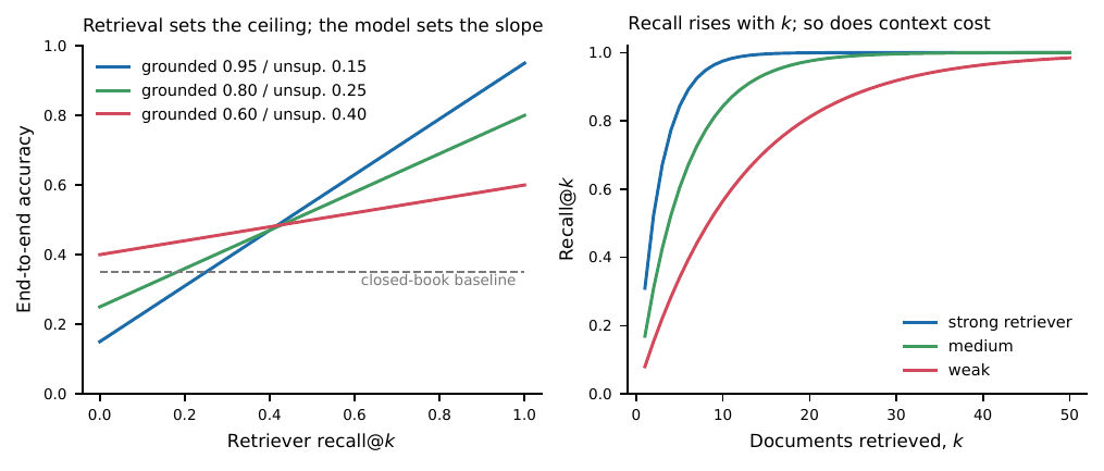
Figure 1:The retriever, not the prompt, sets the ceiling. Left: the equation for three generator profiles. Systems with a high grounded accuracy gain most from better retrieval, and below a crossing point they perform worse than a model answering from memory alone, because retrieved-but-irrelevant context displaces what the model knows. Right: recall@ against for three retriever qualities under a simple rank model. A weak retriever can be rescued by a larger , but only at the cost of context length, latency and the dilution the left panel warns about. :width: 90%
The reason to belabour the equation is that in practice is usually the binding constraint, and the three numbers a builder should always report make that visible: recall@ (the retriever’s ), grounded accuracy (, correctness when the evidence was retrieved), and the unsupported-answer rate (how often the system answers confidently with no supporting passage in context). The illustrative run in Example retrieval_augmented_generation-3, which simulates a corpus with a plausible rank model rather than reporting any particular product’s benchmark, is representative of the pattern: at the retriever recovers the supporting passage about four times in five, grounded accuracy is high, and end-to-end accuracy sits well below grounded accuracy purely because the missing fifth of retrievals drags it down. The lesson is not the specific figures --- which depend on the corpus, the encoder and the questions, and would be meaningless quoted out of that context --- but their ordering: end-to-end accuracy tracks far more closely than it tracks any property of the generator, so a builder who measures only end-to-end accuracy cannot tell an improvable retrieval problem from a generation ceiling. Report all three, and report recall first, because it is the number most likely to be the one holding the system back. Because recall rises with while a longer context is harder to use, end-to-end accuracy is a product of an increasing and a decreasing factor. Sweeping shows the shape that the term of the equation predicts.
import numpy as np
rng = np.random.default_rng(0)
nq = 4000
print("  k   recall@k   P(correct | retrieved)   end-to-end accuracy")
for k in [1, 2, 3, 5, 10, 20, 40]:
    r = 1 - 0.72**k                                        # more passages, better recall
    pg = 0.92 * 0.97**(k - 1)                              # ...but a longer, noisier context
    got = rng.random(nq) < r
    acc = np.where(got, rng.random(nq) < pg, rng.random(nq) < 0.18).mean()
    print(f"{k:3d}     {r:.3f}            {pg:.3f}                 {acc:.3f}")
print("recall is monotone in k; accuracy is not -- it peaks and then decays as context is stuffed")
k recall@k P(correct | retrieved) end-to-end accuracy
1 0.280 0.920 0.384
2 0.482 0.892 0.511
3 0.627 0.866 0.615
5 0.807 0.814 0.683
10 0.963 0.699 0.676
20 0.999 0.516 0.525
40 1.000 0.280 0.307
recall is monotone in k; accuracy is not -- it peaks and then decays as context is stuffedRecall is monotone in and accuracy is not: it peaks around and then falls, even though the evidence is present more often. Reporting recall@ alone therefore recommends the wrong . This is a bias--variance trade-off in disguise, with context length as the complexity parameter and the optimum well short of “retrieve everything”.
Position effects are measurable without any new data: hold the retrieved passages fixed and permute their order. Evidence in the middle of the context is used less often than evidence at either end, so accuracy depends on an ordering nobody reported.
import numpy as np
rng = np.random.default_rng(0)
nq, k, B = 300, 5, 10                                      # 5 passages, 10 orderings each
use = np.array([0.90, 0.68, 0.62, 0.66, 0.86])             # P(use evidence) by slot: ends beat middle
u = rng.random(nq)                                         # per-question propensity, fixed across orderings
ans = np.array([u < use[rng.integers(0, k, nq)] for _ in range(B)]).T
per = ans.mean(0)
print("accuracy by ordering:", np.round(per, 3))
print(f"mean {per.mean():.3f}   SD across orderings {per.std(ddof=1):.4f}   range {per.max()-per.min():.3f}")
print(f"binomial SE from a single ordering at n=300: {np.sqrt(per.mean()*(1-per.mean())/nq):.4f}")
print(f"questions whose answer flips on reordering alone: {(ans.min(1) != ans.max(1)).mean():.3f}")
print(f"slot means over all runs: {np.round(use, 2)} -- the middle three are the penalty")
accuracy by ordering: [0.647 0.677 0.72 0.673 0.687 0.73 0.653 0.71 0.703 0.68 ]
mean 0.688 SD across orderings 0.0275 range 0.083
binomial SE from a single ordering at n=300: 0.0267
questions whose answer flips on reordering alone: 0.280
slot means over all runs: [0.9 0.68 0.62 0.66 0.86] -- the middle three are the penaltyAccuracy ranges over 8 points across orderings of the same evidence, and the spread across orderings is as large as the binomial standard error from a single run --- so a system evaluated once has an unreported source of variability comparable to its sampling error. Twenty-eight percent of questions flip on order alone. Randomize passage order across evaluation items and report the spread, exactly as a survey statistician rotates item order.
1.3Chunking Is a Design Decision
Splitting documents into retrievable units determines what can be retrieved, and it is made before any modelling. Chunks that are too small lose the context that makes a passage interpretable; chunks that are too large dilute the embedding, so that a single relevant sentence is averaged away by surrounding text. The practical compromise --- moderate chunks with overlap, plus a stored parent pointer so a retrieved chunk can be expanded to its section --- is worth stating explicitly because it is rarely written down. (Orchestration frameworks such as LangChain and LlamaIndex ship this pattern under names like “parent document retriever” and “recursive splitter”; adopting one does not relieve you of choosing the unit, it only supplies a default you did not choose.) The sentence that should make a statistician take chunking seriously is that choosing a chunk is choosing the unit of observation. It is the same decision as deciding whether to analyse at the patient, the visit, or the measurement level: it is made before any modelling, it determines what a single record is, and it constrains every conclusion that can be drawn afterwards. A chunk that is too small is a measurement stripped of the context that makes it interpretable; a chunk that is too large is an aggregate in which the one relevant sentence is averaged together with everything around it, so its embedding no longer points at the query --- the effect the example below makes explicit. Concrete starting values are worth having: chunks of roughly 400 to 800 tokens with 10 to overlap, plus a stored pointer from each chunk back to its parent section so a retrieved chunk can be expanded when the answer needs surrounding context. But these are starting values, not defaults to be trusted --- like any choice of analysis unit they must be tuned against the evaluation set, because the right unit depends on how information is distributed in your particular corpus.
Structured and scientific documents break naive chunkers, and for a statistics readership working mostly from PDFs this is the first thing that will go wrong. A character- or token-count splitter that works acceptably on running prose will cut a table in half, separating a row of numbers from its header; it will strand a figure caption from the figure it describes; it will split a multi-line equation across two chunks so that neither is interpretable; and it will slice a reference list into fragments that retrieve as though they were content. Each of these produces a chunk that embeds and retrieves like ordinary text but carries corrupted or decontextualized information, and none is visible to a retrieval metric, because the chunk is retrieved and is on topic --- it simply pairs the wrong numbers or drops the context that gave them meaning. The practical consequence is that document extraction and structure-aware chunking, treated at length in the tools section below, are not preprocessing niceties but the stage where a scientific RAG system most often fails silently, and they deserve validation before any downstream evaluation is believed. Chunking is the choice of the unit of analysis, and its effect on retrieval is mechanical: a chunk embedding is roughly an average of its sentences, so a long chunk averages the answer together with whatever surrounds it. One sentence answers the query; only the chunk size changes.
import numpy as np
rng = np.random.default_rng(0)
d, T, S = 16, 6, 10                                        # 6 topics of 10 sentences, in order
cent = rng.normal(0, 1, (T, d))
cent[0] = -cent[1]                                         # topic 0 opposes topic 1: averaging cancels
cent[4] = 0.90 * cent[1] + 0.44 * rng.normal(0, 1, d)      # topics 4 and 5 sit near topic 1
cent[5] = 0.90 * cent[1] + 0.44 * rng.normal(0, 1, d)
sent = np.repeat(cent, S, axis=0) * 2.2 + rng.normal(0, 1, (T * S, d))
key = 17                                                    # the sentence answering the query
q = sent[key] + 0.9 * rng.normal(0, 1, d)
unit = lambda A: A / np.linalg.norm(A, axis=-1, keepdims=True)
print(" chunk size   #chunks   rank of the chunk holding the answer   its cosine")
for cs in [1, 2, 5, 10, 20, 30]:
    ch = sent.reshape(-1, cs, d).mean(1)                    # a chunk embedding averages its sentences
    s = unit(ch) @ unit(q)
    hit = key // cs
    print(f"{cs:9d}   {len(ch):7d}   {int(np.where(np.argsort(-s) == hit)[0][0]) + 1:36d}   {s[hit]:10.3f}")
print("once a chunk straddles the topic boundary the answer is averaged away and a coherent neighbour wins")
chunk size #chunks rank of the chunk holding the answer its cosine
1 60 1 0.888
2 30 1 0.847
5 12 1 0.808
10 6 1 0.773
20 3 2 0.533
30 2 2 0.264
once a chunk straddles the topic boundary the answer is averaged away and a coherent neighbour winsCosine to the answer-bearing chunk falls monotonically, and past 20 sentences the correct chunk is no longer ranked first --- it is beaten by a chunk that is uniformly on-topic but contains nothing. Choosing the retrieval unit is the same decision as choosing between patient-, visit-, and measurement-level analysis, and like that decision it is made once, silently, and determines what can be found.
1.4Evaluating a RAG System
Evaluation must be layered, because the two stages fail differently. At the retrieval layer, use the ranking measures of the previous section on a set of questions with known supporting passages. At the generation layer, score faithfulness --- whether each assertion in the answer is entailed by the retrieved context --- separately from correctness, since the two come apart in both directions. A faithful summary of an irrelevant passage is wrong; a correct answer the model produced from memory while ignoring the context is right for the wrong reason and will not generalize to your next corpus. If a model is used as the judge of faithfulness, its agreement with human adjudication must itself be estimated on a subsample, with a or a simple agreement rate. (Packaged RAG evaluation suites such as RAGAS Es et al., 2023 compute faithfulness, answer relevance and context precision for you, but they compute them with a model judge, so the agreement estimate is a prerequisite for reading their output, not an optional extra.) Be concrete about the arithmetic, because the golden set is almost always too small for the comparison it is asked to support. A typical developer-written evaluation set has 20 to 50 questions, and at 50 questions the standard error of an accuracy near 0.6 is about 7 percentage points, so the standard error of a difference between two systems is around 10 points and a gap smaller than about 15 points is not distinguishable from zero. Most reported RAG improvements are smaller than that. The cheapest available remedy is the one the whole evaluation chapter keeps returning to: score both systems on identical questions and report the paired difference, so that the shared difficulty of each question cancels instead of inflating the error term. Example retrieval_augmented_generation-8 shows the paired interval coming in appreciably narrower than the unpaired one on the same data, and it also shows the sobering sample size --- several hundred questions --- needed to resolve a five-point difference even with pairing. The benchmarks section of the evaluation chapter develops the power calculation and the design-effect corrections in full; the point to carry here is that a 30-question golden set cannot adjudicate the differences RAG papers routinely claim, and the honest report is a paired difference with an interval, not two bare accuracies. Faithfulness and correctness are different measurements and they come apart in both directions. Simulating 500 answers with known support and known truth gives the joint distribution that a single accuracy number hides.
import numpy as np
rng = np.random.default_rng(0)
n = 500
supported = rng.random(n) < 0.70                           # the context entails the claim
true_fact = rng.random(n) < 0.65                           # the claim is actually true
faithful = np.where(supported, rng.random(n) < 0.90, rng.random(n) < 0.25)
correct = np.where(faithful, true_fact, rng.random(n) < 0.30)
print(f"faithfulness rate = {faithful.mean():.3f}")
print(f"correctness rate  = {correct.mean():.3f}")
print(f"faithful AND wrong (right answer to a wrong document) = {np.mean(faithful & ~correct):.3f}")
print(f"unfaithful AND right (answered from memory)           = {np.mean(~faithful & correct):.3f}")
tab = np.array([[np.sum(faithful & correct), np.sum(faithful & ~correct)],
                [np.sum(~faithful & correct), np.sum(~faithful & ~correct)]])
print("2x2 table [faithful/not] x [correct/not]:", tab.tolist())
print(f"correlation between the two labels = {np.corrcoef(faithful, correct)[0,1]:.3f}")
faithfulness rate = 0.688
correctness rate = 0.522
faithful AND wrong (right answer to a wrong document) = 0.266
unfaithful AND right (answered from memory) = 0.100
2x2 table [faithful/not] x [correct/not]: [[211, 133], [50, 106]]
correlation between the two labels = 0.272A quarter of the answers are faithful and wrong --- accurate summaries of an unhelpful passage --- and a tenth are correct while ignoring the context, which is the model answering from memory and will not survive a change of corpus. The two labels correlate at only 0.27, so neither is a proxy for the other, and a system reported on correctness alone may be right for a reason that does not generalize.
If a language model adjudicates faithfulness, its agreement with human judgement is itself an estimate with a standard error. Score the same items both ways and compute on subsamples of the size people actually adjudicate.
import numpy as np
rng = np.random.default_rng(0)
n = 300
truth = rng.random(n) < 0.70                               # the claim really is supported
judge = np.where(truth, rng.random(n) < 0.88, rng.random(n) < 0.22)   # LLM judge
human = np.where(truth, rng.random(n) < 0.93, rng.random(n) < 0.08)   # human adjudication
for m in [30, 100, 300]:
    a, b = judge[:m], human[:m]
    po = (a == b).mean()
    pe = a.mean() * b.mean() + (1 - a.mean()) * (1 - b.mean())
    kap, se = (po - pe) / (1 - pe), np.sqrt(po * (1 - po) / m) / (1 - pe)
    print(f"m={m:3d}  agreement {po:.3f}  kappa {kap:.3f}  approx 95% CI [{kap-1.96*se:.3f}, {kap+1.96*se:.3f}]")
print(f"judge-scored faithfulness {judge.mean():.3f} vs human-scored {human.mean():.3f}")
print("the judge's own error rate must be estimated before its score can be reported")
m= 30 agreement 0.833 kappa 0.634 approx 95% CI [0.341, 0.927]
m=100 agreement 0.820 kappa 0.610 approx 95% CI [0.446, 0.773]
m=300 agreement 0.830 kappa 0.635 approx 95% CI [0.543, 0.726]
judge-scored faithfulness 0.623 vs human-scored 0.640
the judge's own error rate must be estimated before its score can be reportedAt --- a typical hand-checked subsample --- the interval on runs from 0.34 to 0.93, which is compatible with anything from fair to near-perfect agreement. The judge’s headline faithfulness rate differs from the human rate by only two points, but that comparison means nothing until the agreement is pinned down, and pinning it down takes a few hundred adjudicated items.
The arithmetic of a small evaluation set determines what a comparison can conclude, and scoring both systems on identical questions is the cheapest variance reduction available.
import numpy as np
rng = np.random.default_rng(0)
Q = 50
print("questions   accuracy A   accuracy B   unpaired 95% CI on diff   paired 95% CI on diff")
for Q in [50, 200]:
    hard = rng.random(Q) < 0.4                             # shared difficulty across systems
    a = np.where(hard, rng.random(Q) < 0.30, rng.random(Q) < 0.85)
    b = np.where(hard, rng.random(Q) < 0.40, rng.random(Q) < 0.92)
    d = b.astype(float) - a
    up = 1.96 * np.sqrt(a.mean()*(1-a.mean())/Q + b.mean()*(1-b.mean())/Q)
    pp = 1.96 * d.std(ddof=1) / np.sqrt(Q)
    print(f"{Q:9d}   {a.mean():10.3f}   {b.mean():10.3f}   [{d.mean()-up:+.3f}, {d.mean()+up:+.3f}]"
          f"          [{d.mean()-pp:+.3f}, {d.mean()+pp:+.3f}]")
print(f"n for a paired half-width of 0.05 at this SD: {int(np.ceil((1.96*d.std(ddof=1)/0.05)**2))}")
questions accuracy A accuracy B unpaired 95% CI on diff paired 95% CI on diff
50 0.580 0.780 [+0.021, +0.379] [+0.052, +0.348]
200 0.660 0.725 [-0.025, +0.155] [-0.009, +0.139]
n for a paired half-width of 0.05 at this SD: 434With 50 questions the unpaired interval on the difference is 0.36 wide; the paired interval is narrower because shared question difficulty cancels. At 200 questions the difference between the systems is no longer distinguishable from zero under either analysis --- the 50-question result was a small sample flattering a small effect. Reaching a paired half-width of 5 points here needs about 434 questions, an order of magnitude more than a typical golden set.
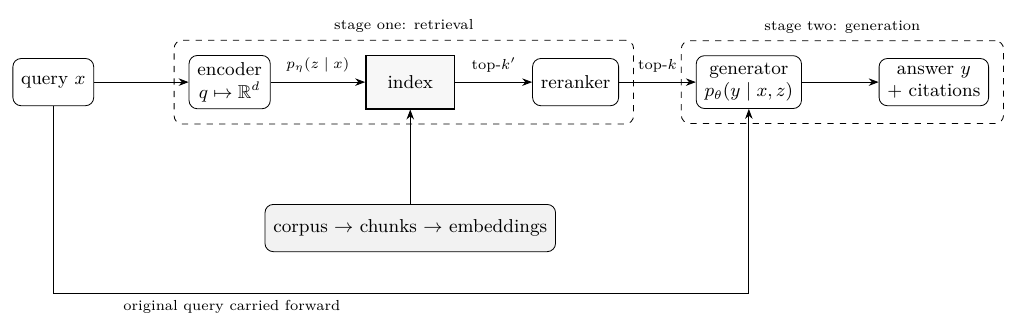
Figure 2:The anatomy of a retrieval-augmented system, drawn to separate the two stages of the equation. Everything to the left of the dashed boundary determines which evidence the generator ever sees, and therefore caps end-to-end accuracy through the term in the equation; everything to the right can only make use of what arrived. The offline path along the bottom --- chunking and embedding the corpus --- is where the design decisions with the largest effect are made. :width: 90%
The primary sources for this section are readily traced. The technique itself was introduced by Lewis et al. (2020), which coined the term and set out the marginal-over-retrievals view of the equation; the dense retriever that made it work in practice, trained to embed questions and passages into a shared space where relevant pairs are close, is dense passage retrieval Karpukhin et al., 2020. Underneath these sit the components developed elsewhere in this book: the contrastive objective that trains a retriever to separate relevant from irrelevant passages Oord et al., 2018, the transformer encoder that produces the passage and query embeddings Devlin et al., 2019, the in-context conditioning that lets a general model use retrieved text without any weight update Brown et al., 2020, and the text-to-text formulation that casts question answering as mapping an input string to an output string Raffel et al., 2020. A reader who understands those four components already understands every moving part of a RAG system; Lewis et al. (2020) and Karpukhin et al. (2020) only assemble them.
1.5Tools in Practice
A RAG system has more moving parts than anything else in this chapter, and correspondingly more places to accept a default without noticing. The categories below follow the pipeline of Figure the figure from left to right, ending with the layer that most implementations skip.
[Document extraction and layout parsing] Corpus preparation. Convert PDFs and office documents into text with structure preserved --- reading order, column boundaries, table cells, figure captions. Fits: the offline path along the bottom of Figure the figure, before chunking. Watch: this is where scientific corpora fail first, and it fails silently: a two-column paper read in raw line order interleaves the columns, and a table read without cell coordinates pairs labels with the wrong numbers. No retrieval metric in this section can detect either, as the example below shows.
[Chunking and orchestration frameworks] Pipeline assembly. LangChain and LlamaIndex supply splitters, retrievers, parent-document expansion and the glue between index and generator. Fits: getting a working pipeline quickly, and standardizing one across a group. Watch: every default is a decision you did not make --- chunk size, overlap, , the fusion rule. Read them out of the configuration and record them next to your results; they move accuracy more than the choice of generator does.
[Hybrid retrieval and fusion] Stage-one recall. Run a dense and a lexical ranker Robertson & Zaragoza, 2009 and fuse by reciprocal rank, as in Section that section. Fits: corpora containing identifiers, which in a statistical or biomedical setting is all of them. Watch: fusion needs no score calibration, which is its main virtue, but it does need both rankers to be evaluated separately. A fused system whose lexical half is broken looks merely mediocre rather than broken.
[Citation-bearing generation] Attribution. Prompting or decoding patterns that require each sentence to name the passage supporting it, so the output can be audited against the retrieved context. Fits: anything you will quote in writing. Watch: a passage identifier attached to a sentence is a claim, not a verification. The mechanism to check it is the same one used for citations in a research report; see Section that section.
[RAG evaluation suites] Layered scoring. Frameworks that score faithfulness, answer relevance and context precision on a question set Es et al., 2023. Fits: the layered evaluation this section argues for, once you have a question set with known supporting passages. Watch: the scorer is a model. Its agreement with human adjudication is an unknown parameter of your evaluation, and Example
retrieval_augmented_generation-7shows how many adjudicated items it takes to pin down.[Tracing and per-item logging] Provenance. Record, for every question, the retrieved passage identifiers, their scores, the assembled prompt and the answer. Fits: the debugging loop, and the paired comparisons of Example
retrieval_augmented_generation-8. Watch: without per-item retrieval logs you cannot compute in the equation, and without you cannot tell whether a disappointing system has a retrieval problem or a generation problem --- which is the first question to answer and the one an aggregate score never answers.
An agent that runs its own multi-step search over an open corpus, rather than answering from a fixed retrieved context, changes the estimand again and introduces a verification problem of its own; Section that section treats it.
The extraction layer deserves a measurement of its own because its errors are invisible downstream. Consider a results table read by a parser that recovers the text but not the cell coordinates: it emits a stream of row labels and a stream of numbers, and pairs them by position. A single label that wraps onto two printed lines inserts one spurious label and shifts every subsequent pairing by one.
import numpy as np
rng = np.random.default_rng(0)
R = 24                                              # a results table with 24 rows
labels = [f"row{r:02d}" for r in range(R)]
values = np.round(rng.normal(0.5, 0.2, R), 3)
def extract(p_wrap):
    # A layout-unaware reader emits a label stream and a value stream, then pairs them
    # by position.  A label that wraps onto two printed lines adds a spurious label.
    lab = []
    for r in range(R):
        lab.append(labels[r])
        if rng.random() < p_wrap:
            lab.append("(cont.)")                   # the wrapped remainder of a long label
    return list(zip(lab, list(values) + [np.nan] * (len(lab) - R)))
print(" P(label wraps)   pairs recovered   correctly paired   first row misread")
for p in [0.0, 0.05, 0.15, 0.40]:
    acc, first = [], []
    for _ in range(2000):
        pairs = extract(p)
        ok = np.array([l == labels[k] and v == values[k]
                       for k, (l, v) in enumerate(pairs[:R])])
        acc.append(ok.mean())
        first.append(R if ok.all() else int(np.argmin(ok)))
    print(f"{p:14.2f}   {R:15d}   {np.mean(acc):16.3f}   {np.mean(first):17.1f}")
print("a layout-aware extractor keeps cell coordinates, so pairing is exact at every wrap rate")
P(label wraps) pairs recovered correctly paired first row misread
0.00 24 1.000 24.0
0.05 24 0.592 14.2
0.15 24 0.275 6.6
0.40 24 0.106 2.5
a layout-aware extractor keeps cell coordinates, so pairing is exact at every wrap rateA wrap probability of 0.05 --- one label in twenty running long, which is unremarkable in a real results table --- leaves only 59% of label--value pairs correct, and the first error arrives around row 14. At 0.15 the majority of the table is wrong. The number of extracted pairs is right in every row of the output, so a pipeline that counts records rather than checking them reports full success. Nothing in the retrieval evaluation of this section detects this: the passage is retrieved, it is on topic, and the number inside it belongs to a different row.
Two lessons follow. The first is that extraction quality belongs in the error decomposition of the equation alongside , because a passage that is retrieved but corrupted contributes to for a reason no amount of prompt work can repair. The second is procedural: validate the extractor before evaluating the system, by hand-checking a random sample of extracted records against the source document and reporting that agreement rate. It is the same instrument-validation step you would insist on before analysing data from an automated assay, and for the same reason --- the downstream analysis cannot see the instrument’s error, so it will report it as a substantive finding.
1.6Exercises
Starting from the equation, show that concatenating the top- passages into a single prompt is not in general equal to the mixture, and describe a situation --- two retrieved passages that contradict each other --- where the two give qualitatively different answers.
Using the equation, derive the condition on , and under which adding retrieval makes accuracy worse than a closed-book model. Interpret it in one sentence.
You measure recall@5 on 40 evaluation questions. Give a 95% interval for the true recall. How many questions would you need for a half-width of 5 percentage points?
Computational. Build a small RAG system over 200 abstracts of your choosing. Sweep and plot both recall@ and end-to-end answer accuracy on a fixed question set. Identify the at which accuracy stops improving and explain the gap between the two curves using the equation.
Computational. Take a fixed retrieved context of five passages and permute their order ten times, holding everything else constant. Report the distribution of answers. Does position affect the result, and how would you report that sensitivity in a paper?
- Liu, N. F., Lin, K., Hewitt, J., Paranjape, A., Bevilacqua, M., Petroni, F., & Liang, P. (2023). Lost in the Middle: How Language Models Use Long Contexts.
- Es, S., James, J., Espinosa-Anke, L., & Schockaert, S. (2023). Ragas: Automated Evaluation of Retrieval Augmented Generation. arXiv Preprint arXiv:2309.15217.
- Lewis, P., Perez, E., Piktus, A., Petroni, F., Karpukhin, V., Goyal, N., Küttler, H., Lewis, M., tau Wen-Yih, Rocktäschel, T., Riedel, S., & Kiela, D. (2020). Retrieval-Augmented Generation for Knowledge-Intensive NLP Tasks.
- Karpukhin, V., Oğuz, B., Min, S., Lewis, P., Wu, L., Edunov, S., Chen, D., & Yih, W. (2020). Dense Passage Retrieval for Open-Domain Question Answering. Proceedings of the 2020 Conference on Empirical Methods in Natural Language Processing (EMNLP), 6769–6781. 10.18653/v1/2020.emnlp-main.550
- van den Oord, A., Li, Y., & Vinyals, O. (2018). Representation Learning with Contrastive Predictive Coding.
- Devlin, J., Chang, M.-W., Lee, K., & Toutanova, K. (2019). BERT: Pre-training of Deep Bidirectional Transformers for Language Understanding.
- Brown, T. B., Mann, B., Ryder, N., Subbiah, M., Kaplan, J., Dhariwal, P., Neelakantan, A., Shyam, P., Sastry, G., Askell, A., Agarwal, S., Herbert-Voss, A., Krueger, G., Henighan, T., Child, R., Ramesh, A., Ziegler, D. M., Wu, J., Winter, C., … Amodei, D. (2020). Language Models are Few-Shot Learners.
- Raffel, C., Shazeer, N., Roberts, A., Lee, K., Narang, S., Matena, M., Zhou, Y., Li, W., & Liu, P. J. (2020). Exploring the Limits of Transfer Learning with a Unified Text-to-Text Transformer.
- Robertson, S., & Zaragoza, H. (2009). The Probabilistic Relevance Framework: BM25 and Beyond. Foundations and Trends® in Information Retrieval, 4(1–2), 1–174. 10.1561/1500000019