import numpy as np
rng = np.random.default_rng(0)

# Three "topics" as orthogonal directions in a 50-dim embedding space.
d = 50
topics = np.linalg.qr(rng.normal(size=(d, 3)))[0].T       # 3 x d, orthonormal
labels = np.repeat(["genomics", "climate", "econometrics"], 4)
docs = np.array([topics[i] + 0.6 * rng.normal(size=d) / np.sqrt(d)
                 for i in np.repeat([0, 1, 2], 4)])
docs /= np.linalg.norm(docs, axis=1, keepdims=True)

S = docs @ docs.T                                         # cosine: rows are unit norm
same = np.equal.outer(labels, labels) & ~np.eye(12, dtype=bool)
print(f"mean cosine within topic : {S[same].mean():+.3f}")
print(f"mean cosine across topics: {S[~np.equal.outer(labels, labels)].mean():+.3f}")
print(f"min within / max across  : {S[same].min():+.3f} / "
      f"{S[~np.equal.outer(labels, labels)].max():+.3f}")
mean cosine within topic : +0.719
mean cosine across topics: -0.030
min within / max across : +0.638 / +0.150import numpy as np
rng = np.random.default_rng(1)
d = 50
topics = np.linalg.qr(rng.normal(size=(d, 3)))[0].T
corpus = np.array([topics[i] + 0.9 * rng.normal(size=d) / np.sqrt(d)
for i in np.repeat([0, 1, 2], 5)])
corpus /= np.linalg.norm(corpus, axis=1, keepdims=True)
names = [f"{t}-{j}" for t in ["gen", "cli", "eco"] for j in range(5)]
query = topics[0] + 0.9 * rng.normal(size=d) / np.sqrt(d) # a genomics query
query /= np.linalg.norm(query)
sims = corpus @ query
order = np.argsort(-sims)[:5]
for r, i in enumerate(order, 1):
mark = "" if names[i].startswith("gen") else " <-- off-topic"
print(f"{r}. {names[i]:<8} cos={sims[i]:+.3f}{mark}")
print(f"\nprecision@5 = {sum(names[i].startswith('gen') for i in order)}/5")1. gen-3 cos=+0.679
2. gen-1 cos=+0.572
3. gen-4 cos=+0.550
4. gen-2 cos=+0.501
5. eco-3 cos=+0.356 <-- off-topic
precision@5 = 4/51Embeddings and Semantic Search
An embedding is a map from an object --- a sentence, a document, an image, a patient record --- to a point in , fitted so that distance in that space tracks similarity of meaning. Statisticians have been building such maps since Hotelling: principal components, classical multidimensional scaling, correspondence analysis and factor scores all produce coordinates whose geometry is supposed to carry substantive information. What is new is not the idea but the source of the geometry, which is now learned from a discriminative objective on enormous unlabelled corpora rather than from an eigendecomposition of a covariance matrix. The practical consequence is that a similarity search over millions of documents becomes a nearest-neighbour query in a few hundred dimensions, and the whole apparatus of retrieval --- which underpins the retrieval-augmented generation of the next section --- reduces to a problem you can reason about with familiar tools. This section covers what the coordinates mean, why cosine similarity is the standard metric, how approximate search buys speed by giving up exactness, and how to evaluate a retrieval system as the diagnostic-test problem it really is.
Table 1:Embeddings and vector search restate multivariate analysis and nearest-neighbour methods in the vocabulary of information retrieval; the last column collects the places where that restatement misleads.
| ML / AI term | Statistical analogue | What is the same | What is different / the catch |
|---|---|---|---|
| Embedding vector | Factor scores; principal component scores; MDS coordinates | A low-dimensional numeric summary of a complex object | Learned from a discriminative objective, not from a covariance structure; coordinates are not identified |
| Embedding dimension | Number of retained components | Controls how much structure the representation can carry | Chosen by the model vendor, not by a scree plot; no variance-explained interpretation |
| Cosine similarity | Correlation between two centred vectors; direction cosine | Scale-invariant measure of alignment | Equals correlation only after centring; embeddings are usually not centred |
| Semantic search | -nearest-neighbour query under a learned metric | Retrieve the closest points to a query | The metric is estimated and task-dependent, so “closest” inherits the training objective |
| Vector database / index | A spatial data structure (k-d tree, ball tree) | Sublinear neighbour lookup | Exact trees fail in high ; production indexes are deliberately approximate |
| Approximate nearest neighbour (HNSW, IVF) | A sampling or screening design for a search | Examine a fraction of candidates | Introduces a recall--latency trade-off you must measure, not assume |
| Contrastive / InfoNCE objective | Conditional logistic regression on matched sets; case--control sampling | Score the true match against sampled alternatives | The “negatives” are a design choice that determines what similarity means |
| Bi-encoder | Two separate feature maps compared by inner product | Separable scoring; precomputable | Cannot model interactions between query and document |
| Cross-encoder / reranker | A model with the interaction term included | Higher fidelity scoring | Costs model calls, so it is used only on a short list |
| Chunking | Choosing the unit of observation | Defines what a “case” is | An analysis decision disguised as preprocessing; changes recall more than the model does |
| Recall@ | Sensitivity of a screening test at a fixed referral rate | Fraction of true positives captured | Reported without an interval, on very few queries |
| Curse of dimensionality | Concentration of distances in high | Neighbours become less distinguishable | Real embeddings live on a low-dimensional manifold, so the pessimistic theory does not bind |
| Hubness | A few points that are everyone’s neighbour | Analogous to high-leverage observations | Specific to high- neighbour graphs; fixed by centring or similarity normalization |
1.1From Counts to Learned Coordinates
The oldest text representations are counts, and the classical route from counts to coordinates is a factorization: a truncated singular value decomposition of a term--document matrix is latent semantic analysis, and it is PCA in disguise. Neural embeddings replaced the decomposition with a prediction task --- predicting a word from its context Bengio et al., 2003 --- and then replaced static per-word vectors with context-dependent ones produced by a transformer encoder Devlin et al., 2019. The modern sentence embedding is one of those contextual models with a pooling step and a contrastive fine-tuning stage on paired data. It is worth tracing the arc from counts to sentence encoders, because every step on it is a statistician’s move made under a different name. Latent semantic analysis was an explicit factorization: a truncated singular value decomposition of a term--document matrix, which is principal components applied to counts, with the retained left singular vectors serving as coordinates. word2vec Bengio et al., 2003 and GloVe Pennington et al., 2014 then replaced the explicit decomposition with a prediction task --- predict a word from its context, or fit log co-occurrence counts --- and produced dense per-word vectors as a by-product. The apparent break from the factorization tradition is smaller than it looks: Levy & Goldberg (2014) showed that word2vec’s skip-gram objective is implicitly factorizing a shifted pointwise-mutual-information matrix, so the neural method and the SVD method are computing coordinates for essentially the same matrix by different numerical routes. The middle example below does this factorization explicitly to make the equivalence concrete.
The next two steps continue the same substitution. Static word vectors gave one coordinate per word regardless of context, so “bank” had a single embedding; contextual encoders such as BERT Devlin et al., 2019 produce a different vector for each occurrence, which is again an implicit factorization --- now of a context-conditioned co-occurrence structure realized by a transformer rather than written down as a matrix. Sentence embeddings add a final stage: take a contextual encoder, pool its token vectors into one vector per sentence, and fine-tune with a contrastive objective on paired data so that paraphrases land near each other. Each step of the arc replaced an explicit matrix factorization with an implicit one learned from a harder prediction task, and each bought context-sensitivity at the cost of an interpretable spectrum. The reader who is comfortable with PCA has already met the first step and, through Levy & Goldberg (2014), a version of the second; the rest is the same idea carried through more expressive models. Latent semantic analysis is a truncated SVD of a term--document matrix, so the whole idea of a learned coordinate can be shown on a six-document corpus. Compare raw count-vector cosines with cosines in the two-dimensional LSA space.
import numpy as np
terms = ["power", "sample", "size", "gpu", "cluster", "throughput"]
docs = ["d1", "d2", "d3", "d4", "d5", "d6"]
X = np.array([[1, 1, 1, 0, 0, 0], [1, 1, 0, 0, 0, 0], [1, 0, 1, 0, 0, 0],
              [1, 0, 0, 1, 1, 0], [1, 0, 0, 0, 1, 1], [0, 0, 0, 1, 1, 1]], float).T
U, s, Vt = np.linalg.svd(X, full_matrices=False)
Z = (U[:, :2] * s[:2])                                  # 2-d term coordinates = LSA embedding
cos = lambda a, b: a @ b / (np.linalg.norm(a) * np.linalg.norm(b))
print(f"raw count-vector cosine, 'size' vs 'throughput' : {cos(X[2], X[5]):.3f}")
print(f"raw count-vector cosine, 'size' vs 'sample'     : {cos(X[2], X[1]):.3f}")
print(f"LSA(2) cosine,           'size' vs 'throughput' : {cos(Z[2], Z[5]):.3f}")
print(f"LSA(2) cosine,           'size' vs 'sample'     : {cos(Z[1], Z[2]):.3f}")
print("singular values:", np.round(s, 3))
print(f"variance-explained analogue of the first 2 components: {(s[:2]**2).sum()/(s**2).sum():.3f}")
raw count-vector cosine, 'size' vs 'throughput' : 0.000
raw count-vector cosine, 'size' vs 'sample' : 0.500
LSA(2) cosine, 'size' vs 'throughput' : -0.081
LSA(2) cosine, 'size' vs 'sample' : 1.000
singular values: [2.929 2.165 1. 1. 0.838 0.188]
variance-explained analogue of the first 2 components: 0.829Two terms that never co-occur have raw cosine exactly zero --- the count representation cannot see that they are related --- while in the truncated space they align, because they load on the same component. That is the entire proposition of an embedding, and it is a rank-reduction argument the reader already accepts in the principal-components setting.
The next step in the arc replaces the explicit factorization with a prediction task, but the object being factorized can be written down: word2vec’s objective is implicitly factorizing a shifted pointwise-mutual-information matrix. Here we do it explicitly, with an SVD of the SPPMI matrix computed from co-occurrence counts.
import numpy as np
rng = np.random.default_rng(0)
V, T = 12, 300000
emit = np.array([[.30, .30, .20, .10, .05, .05, 0, 0, 0, 0, 0, 0],
                 [0, 0, 0, 0, .05, .05, .30, .30, .20, .10, 0, 0],
                 [.05, 0, 0, 0, 0, 0, 0, 0, .10, .20, .30, .35]])
z = np.repeat(rng.integers(0, 3, T // 20), 20)             # topics persist over 20-word runs
w = np.array([rng.choice(V, p=emit[t]) for t in z])
C = np.zeros((V, V)); np.add.at(C, (w[:-1], w[1:]), 1.0)   # co-occurrence counts
P = C / C.sum()
PMI = np.log(np.maximum(P, 1e-12) / np.outer(P.sum(1), P.sum(0)))
SPPMI = np.maximum(PMI - np.log(1.0), 0)                   # shifted positive PMI, shift k=1
U, s, _ = np.linalg.svd(SPPMI)
E = U[:, :3] * np.sqrt(s[:3])                              # word2vec-style vectors, via SVD
cs = lambda a, b: a @ b / (np.linalg.norm(a) * np.linalg.norm(b))
print(f"cosine(word0, word1)  both topic 0        = {cs(E[0], E[1]):+.4f}")
print(f"cosine(word6, word7)  both topic 1        = {cs(E[6], E[7]):+.4f}")
print(f"cosine(word0, word7)  topic 0 vs topic 1  = {cs(E[0], E[7]):+.4f}")
print(f"share of squared spectrum in 3 components = {(s[:3]**2).sum()/(s**2).sum():.3f}")
print(f"cosine(word0, word4)  word4 straddles topics = {cs(E[0], E[4]):+.4f}")
cosine(word0, word1) both topic 0 = +0.9998
cosine(word6, word7) both topic 1 = +1.0000
cosine(word0, word7) topic 0 vs topic 1 = -0.0135
share of squared spectrum in 3 components = 0.990
cosine(word0, word4) word4 straddles topics = +0.7127Words from the same latent topic have cosine near one and words from different topics near zero, with the ambiguous word 4 --- emitted by two topics --- sitting between them. No neural network was trained. The lesson is that “learned” embeddings and classical factor scores are not different species: the objective determines which matrix gets factorized, and the geometry follows from that choice.
1.2The Objective That Creates the Geometry
Most retrieval embeddings are trained with a contrastive loss. Given a query , its true match , and sampled non-matches , the InfoNCE objective Oord et al., 2018Chen et al., 2020 is
which is precisely the conditional logistic likelihood of a matched case--control set: one case, controls, and a score that plays the role of the linear predictor. Reading it that way makes two things obvious. First, the similarity the model learns is defined relative to the negatives you sampled; train against random documents and the model learns topic, train against hard negatives from the same topic and it learns fine distinctions. Second, the temperature controls how sharply the loss penalizes near misses, and the objective is invariant to the norm of the embeddings, which is why cosine rather than Euclidean distance is the natural metric. The matched case--control reading is the single best translation this section offers, so it is worth dwelling on. A matched case--control study fixes a stratum --- a case and the controls matched to it --- and asks the conditional logistic model to score the case above its own controls, conditioning away everything the stratum shares. Equation the equation is that model exactly: the query defines the stratum, is the case, the sampled non-matches are the matched controls, and is the linear predictor. The contrastive encoder is not learning “what a document means” in any absolute sense; it is learning to win a conditional comparison against a particular control group, and the model that comes out is only ever as discriminating as the controls made it be. The consequence for practice is blunt: the question “is this embedding good?” has no answer. The only well-posed question is “good at distinguishing what from what?”, because an embedding trained to separate documents by topic will fail to separate two documents within a topic, and an accuracy measured against easy controls tells you nothing about performance against hard ones. When a vendor reports that an encoder is state of the art, the missing phrase is always the control group, and it is the phrase that decides whether the encoder will work on your retrieval problem. The last example in this subsection makes the dependence on the control group visible by training the same metric against easy and hard negatives and evaluating both on both tasks. Equation the equation is claimed to be a conditional logistic likelihood on matched sets. That claim is checkable: fit InfoNCE directly by numerical minimization, fit conditional logistic regression on the case-minus-control contrasts, and compare the coefficient vectors.
import numpy as np
from scipy.optimize import minimize
from sklearn.linear_model import LogisticRegression
rng = np.random.default_rng(0)
n, M, d = 400, 3, 4                                   # n matched sets: 1 case, 3 controls
beta = np.array([1.0, -0.5, 0.8, 0.3])
S = rng.normal(0, 1, (n, M + 1, d))                   # column 0 is the true match
S[:, 0] += 0.9 * beta / np.linalg.norm(beta)
def infonce(b, shift=0.0):                            # InfoNCE at tau = 1
    z = S @ b + shift
    return -(z[:, 0] - np.log(np.exp(z).sum(1))).mean()
b_nce = minimize(infonce, np.zeros(d)).x
Xd = (S[:, 0:1] - S[:, 1:]).reshape(-1, d)            # case-minus-control contrasts
b_clr = LogisticRegression(fit_intercept=False, C=1e6, max_iter=1000).fit(
    np.vstack([Xd, -Xd]), np.r_[np.ones(len(Xd)), np.zeros(len(Xd))]).coef_[0]
print("InfoNCE argmin              :", np.round(b_nce, 3))
print("conditional-logistic fit    :", np.round(b_clr, 3))
print(f"cosine between the two      : {b_nce@b_clr/np.linalg.norm(b_nce)/np.linalg.norm(b_clr):.4f}")
print(f"loss with score shift +0    : {infonce(b_nce, 0.0):.6f}")
print(f"loss with score shift +10   : {infonce(b_nce, 10.0):.6f}")
InfoNCE argmin : [ 0.529 -0.378 0.528 0.182]
conditional-logistic fit : [ 0.547 -0.38 0.5 0.171]
cosine between the two : 0.9992
loss with score shift +0 : 1.139621
loss with score shift +10 : 1.139621The two coefficient vectors are the same fit to three decimals, and adding a constant to every score leaves the loss unchanged --- the matched-set likelihood conditions the shift away exactly as a stratified analysis eliminates a stratum-specific intercept. The practical consequence is that a contrastive similarity score has no absolute meaning; only comparisons within a candidate set are estimable.
If the negatives define the comparison, then changing the negatives should change what the embedding is good at. We learn a linear metric by stochastic gradient on a contrastive objective, once with negatives drawn from other topics and once with hard negatives from the same topic, and evaluate both on both tasks.
import numpy as np
rng = np.random.default_rng(0)
d, ntop, nsub = 16, 4, 4                                   # 4 topics x 4 subtopics
topic = rng.normal(0, 1, (ntop, d))
sub = topic[:, None, :] + 0.35 * rng.normal(0, 1, (ntop, nsub, d))
def train(hard):
    W = np.eye(d)                                          # learned metric u'W'Wv
    for _ in range(300):
        t, s = rng.integers(0, ntop), rng.integers(0, nsub)
        q = sub[t, s] + 0.15 * rng.normal(0, 1, d)
        pos = sub[t, s]
        neg = sub[t, (s + 1) % nsub] if hard else sub[(t + 1) % ntop, s]
        g = np.outer(W @ (neg - pos), q) + np.outer(W @ q, neg - pos)
        W -= 0.02 * g / (1 + np.linalg.norm(g))
    return W
def acc(W, hard):                                          # can it pick the right neighbour?
    ok = 0
    for _ in range(2000):
        t, s = rng.integers(0, ntop), rng.integers(0, nsub)
        q = W @ (sub[t, s] + 0.15 * rng.normal(0, 1, d))
        alt = W @ (sub[t, (s + 1) % nsub] if hard else sub[(t + 1) % ntop, s])
        ok += q @ (W @ sub[t, s]) > q @ alt
    return ok / 2000
Wr, Wh = train(False), train(True)
print(f"random negatives -> coarse (cross-topic) task : {acc(Wr, False):.3f}")
print(f"random negatives -> fine (within-topic) task  : {acc(Wr, True):.3f}")
print(f"hard negatives   -> coarse (cross-topic) task : {acc(Wh, False):.3f}")
print(f"hard negatives   -> fine (within-topic) task  : {acc(Wh, True):.3f}")
random negatives -> coarse (cross-topic) task : 1.000
random negatives -> fine (within-topic) task : 0.607
hard negatives -> coarse (cross-topic) task : 1.000
hard negatives -> fine (within-topic) task : 0.794Both metrics separate topics perfectly, but only the one trained against hard negatives can tell two documents within a topic apart. The question “is this embedding good?” has no answer: the training negatives are the control group, and a model trained against easy controls has never been asked the hard question.
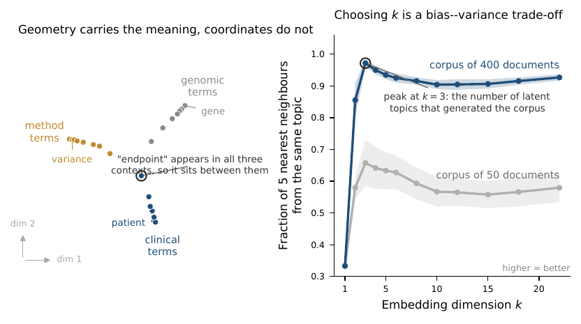
Figure 1:Two facts about vector search that govern how it is deployed. Left: the sampling distribution of the cosine similarity between two independent isotropic vectors concentrates at zero as dimension grows, so in a 768-dimensional space almost all pairs are near-orthogonal and even a modest similarity is a strong signal. Right: recall@10 of a random-projection index on a clustered corpus of 20{,}000 vectors, relative to exact cosine search. Cheap approximate scoring alone loses many true neighbours, but retrieving a longer candidate list and rescoring it exactly recovers most of them --- the retrieve-then-rerank pattern used by every production system. :width: 90%
1.3Cosine Similarity and What It Is Not
For vectors ,
so ranking by cosine similarity and ranking by Euclidean distance on normalized vectors are the same operation --- a fact worth stating because the two are often presented as competing choices. Cosine similarity is Pearson correlation only when the vectors are centred, and embedding vectors typically have a large shared mean direction, which inflates all pairwise similarities and produces the familiar complaint that “everything looks similar”. Subtracting the corpus mean before comparison is a one-line fix that meaningfully improves retrieval. The centring fix is worth demonstrating rather than asserting, because it is the most actionable single tip in the section and costs one line of code. The demonstration to run is the simplest possible one: take an embedding set, report the mean pairwise cosine similarity, subtract the corpus mean direction from every vector, and report the mean pairwise cosine again. The example below does exactly that on a synthetic set built to carry a large shared direction, and also tracks what the shared direction was costing --- the spread of the similarities, the retrieval accuracy, and the worst hub.
Embedding vectors typically share a large common direction, which inflates every pairwise cosine. Subtract the corpus mean and re-measure --- watch the mean similarity, its spread, the retrieval accuracy, and how often a single point turns up as everybody’s nearest neighbour.
import numpy as np
rng = np.random.default_rng(0)
n, d, nq = 600, 64, 300
anchor = rng.normal(0, 1, d)                                # a shared "corpus" direction
E = 3.0 * anchor + rng.normal(0, 1, (n, d))                 # embeddings with a large common mean
unit = lambda A: A / np.linalg.norm(A, axis=-1, keepdims=True)
off = ~np.eye(n, dtype=bool)
for name, A in [("raw", E), ("centred", E - E.mean(0))]:
    Cm = unit(A) @ unit(A).T
    tgt = rng.integers(0, n, nq)
    Q = A[tgt] + 1.6 * rng.normal(0, 1, (nq, d))            # noisy queries for known documents
    top1 = (unit(Q) @ unit(A).T).argmax(1)
    hub = np.bincount((Cm - 2 * np.eye(n)).argmax(1), minlength=n).max()
    print(f"{name:8s}  mean pairwise cos = {Cm[off].mean():+.4f}  SD = {Cm[off].std():.4f}"
          f"  recall@1 = {(top1 == tgt).mean():.3f}  hubness = {hub}")
print("centring removes the shared direction; similarities spread out and the hub shrinks")
raw mean pairwise cos = +0.8830 SD = 0.0204 recall@1 = 0.917 hubness = 22
centred mean pairwise cos = -0.0017 SD = 0.1252 recall@1 = 0.947 hubness = 6
centring removes the shared direction; similarities spread out and the hub shrinksBefore centring the average cosine is 0.88 with almost no spread, so “similarity” has essentially no dynamic range; after centring it is centred at zero, recall@1 improves, and the worst hub is a quarter as dominant. Subtracting the mean is the same standardization step you would apply before any correlation analysis, and it is the cheapest improvement available to a retrieval system.
Equation the equation says cosine and Euclidean rankings agree for unit vectors. The counterexample when they are not normalized fits in two lines, and the same divergence shows up in a real ranking.
import numpy as np
u, v, q = np.array([3.0, 0.0]), np.array([1.0, 0.0]), np.array([0.9, 0.44])
cos = lambda a, b: a @ b / (np.linalg.norm(a) * np.linalg.norm(b))
print(f"cosine(q,u) = {cos(q,u):.4f}  cosine(q,v) = {cos(q,v):.4f}  -> exact tie")
print(f"||q-u|| = {np.linalg.norm(q-u):.4f}  ||q-v|| = {np.linalg.norm(q-v):.4f}  -> v wins on distance")
rng = np.random.default_rng(0)
unit = lambda A: A / np.linalg.norm(A, axis=-1, keepdims=True)
A = rng.normal(0, 1, (200, 8)) * rng.lognormal(0, 1, (200, 1))   # heterogeneous norms
qq = rng.normal(0, 1, 8)
print("top-5 by cosine           :", np.argsort(-(unit(A) @ unit(qq)))[:5])
print("top-5 by Euclidean, raw   :", np.argsort(np.linalg.norm(A - qq, axis=1))[:5])
print("top-5 by Euclidean, unit  :", np.argsort(np.linalg.norm(unit(A) - unit(qq), axis=1))[:5])
cosine(q,u) = 0.8984 cosine(q,v) = 0.8984 -> exact tie
||q-u|| = 2.1456 ||q-v|| = 0.4512 -> v wins on distance
top-5 by cosine : [ 42 167 182 0 44]
top-5 by Euclidean, raw : [ 42 167 181 44 9]
top-5 by Euclidean, unit : [ 42 167 182 0 44]Two collinear vectors of different lengths tie exactly on cosine and differ by a factor of five in distance, and on the random corpus the raw-Euclidean top-5 differs from the other two, which agree exactly. Whether to normalize is a modelling decision about whether vector length carries information; for text embeddings length mostly encodes document length, which is why cosine is the convention.
1.4Search at Scale, and the Recall You Give Up
Exact search over vectors costs per query, which is fine for and unacceptable for . Production indexes are approximate: inverted-file methods partition the space and search only the nearest few cells, graph methods such as HNSW walk a navigable neighbour graph Malkov & Yashunin, 2020, and product quantization compresses vectors so more of them fit in memory. (All three are implemented behind one interface in FAISS Douze et al., 2024, which is the reference implementation most vector databases wrap.) Every one of these exposes a knob that trades recall for latency, and the resulting curve --- not a single number --- is what should be reported. The pattern that resolves most practical complaints about approximate search is retrieve-then-rerank, and it is a two-phase design in the statistical sense. The first phase uses a fast, cheap, deliberately approximate index to return a candidate list of length --- far more than the results the user will see. The second phase scores those candidates with an expensive but accurate function, either exact cosine over the full-precision vectors or a cross-encoder that reads query and document together, and keeps the top . The reason this works is a division of labour between sensitivity and specificity. The first phase only has to be sensitive: it must get the true neighbours somewhere into the candidate list, and it is allowed to rank them badly, because the second phase re-ranks. The second phase supplies the precision, but it only has to score candidates rather than the whole corpus, so its per-query cost is bounded and independent of . The net effect is a final list nearly as good as exhaustive search at a fraction of the cost, and Figure the figure shows the shape of the trade-off: recall climbs steeply with and then flattens, so there is a candidate-list length past which reranking buys nothing. The design has one hard ceiling worth stating in advance --- the reranker can only reorder what the first phase returned, so the best achievable recall@ is the retriever’s own recall@, and no reranker recovers a neighbour the first phase dropped.
Approximate search trades recall for speed, and the trade-off is measurable rather than theoretical. A random-projection sketch gives a cheap Hamming ranking; the question is how much of the exact top-10 survives, and how much of it a rescoring pass recovers.
import numpy as np
rng = np.random.default_rng(0)
n, d, nq, m = 5000, 64, 200, 128                            # m = bits in the random-projection sketch
X = rng.normal(0, 1, (n, d)) + 1.5 * rng.normal(0, 1, (25, d))[rng.integers(0, 25, n)]
X /= np.linalg.norm(X, axis=1, keepdims=True)
Q = X[rng.integers(0, n, nq)] + 0.7 * rng.normal(0, 1, (nq, d))
Q /= np.linalg.norm(Q, axis=1, keepdims=True)
truth = np.argsort(-(Q @ X.T), axis=1)[:, :10]              # exact top-10
R = rng.normal(0, 1, (d, m))
ham = ((Q @ R > 0)[:, None, :] != (X @ R > 0)[None, :, :]).sum(2)
order = np.argsort(ham, axis=1, kind="stable")
rec = lambda lists: np.mean([len(set(a) & set(t)) / 10 for a, t in zip(lists, truth)])
print(f"sketch top-10, no rerank: recall@10 = {rec(order[:, :10]):.3f}")
for kp in [10, 50, 200, 1000]:
    cand = order[:, :kp]
    print(f"k'={kp:5d} ({100*kp/n:5.1f}% of corpus scored exactly)  recall@10 after rerank = "
          f"{rec([c[np.argsort(-(X[c] @ Q[i]))[:10]] for i, c in enumerate(cand)]):.3f}")
sketch top-10, no rerank: recall@10 = 0.123
k'= 10 ( 0.2% of corpus scored exactly) recall@10 after rerank = 0.123
k'= 50 ( 1.0% of corpus scored exactly) recall@10 after rerank = 0.316
k'= 200 ( 4.0% of corpus scored exactly) recall@10 after rerank = 0.597
k'= 1000 ( 20.0% of corpus scored exactly) recall@10 after rerank = 0.921The sketch alone finds barely a tenth of the true neighbours, which would be a disastrous retrieval system. Retrieving a longer candidate list and rescoring it exactly recovers 92% of them while scoring only a fifth of the corpus --- the retrieve-then-rerank pattern of Figure the figure. The first stage needs recall, not precision; precision is the second stage’s job.
Dense retrieval also has a blind spot that matters disproportionately for scientific corpora: exact identifiers --- gene symbols, accession numbers, statute references, a specific -value --- are precisely what an embedding smooths away, and precisely what classical lexical scoring such as BM25 finds trivially Robertson & Zaragoza, 2009. Hybrid search, which fuses a dense ranking with a lexical one, reliably beats either alone. The practical recipe for hybrid search is short and needs no tuning to get started. Run both rankers over the same corpus --- a dense retriever and a lexical BM25 scorer --- so that each query produces two ranked lists. Fuse them by reciprocal rank: give each document a score with a small constant (60 is the usual choice), and re-sort by the fused score. Reciprocal-rank fusion is the right default because it uses only the ranks, not the raw scores, so it sidesteps the problem that a cosine similarity and a BM25 weight live on incomparable scales and cannot simply be added. The check that tells you whether the fusion is earning its place is to look specifically at queries containing an exact identifier --- a gene symbol, an accession number, a statute reference --- because that is where a dense-only system fails most visibly: the embedding smooths the identifier into its neighbourhood and buries the one document that actually contains it, while BM25 finds it in first place. If hybrid search is going to matter for your corpus, those queries are where it shows, and they are worth carving out as a named slice of the evaluation set rather than averaging them into an aggregate that hides the failure.
Dense retrieval smooths, and smoothing is exactly wrong for an exact identifier. Here two queries carry an accession-style identifier and two are paraphrases, with a lexical ranker and a dense ranker each strong on one pair and weak on the other; reciprocal-rank fusion combines them.
import numpy as np
rng = np.random.default_rng(0)
n, gold = 30, [3, 11, 19, 26]                              # 30 documents, 4 queries
sc_lex, sc_den = rng.random((4, n)), rng.random((4, n))
for i, g in enumerate(gold):                               # queries 1-2 carry an identifier,
    win, lose = (sc_lex, sc_den) if i < 2 else (sc_den, sc_lex)   # queries 3-4 are paraphrases
    win[i, g] = 1.5                                        # the suited ranker puts gold first
    lose[i, g] = np.sort(lose[i])[-6] + 1e-6               # the other buries it around rank 6
rank = {"lexical": [], "dense": [], "fused": []}
for i, g in enumerate(gold):
    L, D = np.argsort(-sc_lex[i]), np.argsort(-sc_den[i])
    f = np.zeros(n)
    for r in (L, D):
        for rk, doc in enumerate(r): f[doc] += 1 / (60 + rk + 1)      # reciprocal-rank fusion
    for k, o in [("lexical", L), ("dense", D), ("fused", np.argsort(-f))]:
        rank[k].append(int(np.where(o == g)[0][0]) + 1)
    print(f"query {i+1} ({'identifier' if i < 2 else 'paraphrase'}): gold rank"
          f"  lexical {rank['lexical'][-1]}  dense {rank['dense'][-1]}  fused {rank['fused'][-1]}")
for k, v in rank.items():
    print(f"{k:8s} MRR {np.mean([1/x for x in v]):.3f}   recall@3 {np.mean([x <= 3 for x in v]):.2f}   worst rank {max(v)}")
query 1 (identifier): gold rank lexical 1 dense 6 fused 1
query 2 (identifier): gold rank lexical 1 dense 6 fused 1
query 3 (paraphrase): gold rank lexical 6 dense 1 fused 2
query 4 (paraphrase): gold rank lexical 6 dense 1 fused 1
lexical MRR 0.583 recall@3 0.50 worst rank 6
dense MRR 0.583 recall@3 0.50 worst rank 6
fused MRR 0.875 recall@3 1.00 worst rank 2Each ranker alone has an MRR of 0.58 and a worst-case rank of 6 --- fatal if only the top three passages reach the generator. The fused list keeps every gold document in the top two. Fusion by reciprocal rank needs no score calibration between the two systems, which is what makes it usable when one score is a cosine and the other a BM25 weight.
1.5Evaluating Retrieval as a Diagnostic Test
Retrieval evaluation is screening-test evaluation with a different vocabulary. For a query with relevant set and retrieved list of length ,
where is the graded relevance of the item at rank and its value under the ideal ordering. Recall@ is sensitivity at a fixed referral rate; sweeping traces a curve directly analogous to an ROC curve. Because these are means over queries, they carry standard errors, and with the 30 or 50 queries typical of a homegrown evaluation set those standard errors are large. (Public embedding leaderboards report these same quantities averaged over many public task sets Muennighoff et al., 2022; they are useful for shortlisting an encoder and no substitute for measuring recall on your own corpus, since the training data of a candidate encoder may overlap the leaderboard’s tasks and certainly does not overlap yours.) The sample-size arithmetic deserves to be stated plainly, because it is routinely ignored. A recall@10 estimate is a mean of a outcome over queries, so near 0.5 its standard error is , which at queries is about 0.07. The standard error of the difference between two retrievers scored on independent query sets is then roughly 0.10, so two systems differing by ten points of recall are not distinguishable --- the interval on the difference comfortably covers zero. This is the same underpowered-comparison problem that runs through the whole evaluation chapter, and it has the same cheap remedy: score both retrievers on the same queries and analyse the paired differences. Query difficulty is the dominant source of variance and it is shared within a query, so pairing cancels it, and only the queries on which the two systems actually disagree contribute to the standard error. The example below shows the paired interval coming in appreciably narrower than the unpaired one on the identical data; the recommendation is to always evaluate retrievers on a common query set and report the paired difference, which is the crossover-design argument the reader already knows from clinical trials.
Retrieval metrics are means over queries, so they have standard errors, and the two retrievers are scored on the same queries. Compare the unpaired interval with the paired one.
import numpy as np
rng = np.random.default_rng(0)
Q, pA, delta = 50, 0.60, 0.08                              # 50 evaluation queries
z = rng.random(Q) < 0.75                                   # query difficulty is shared
a = np.where(z, rng.random(Q) < pA / 0.75 * 0.9, rng.random(Q) < 0.15)
b = np.where(z, rng.random(Q) < (pA + delta) / 0.75 * 0.9, rng.random(Q) < 0.15)
se = lambda v: np.sqrt(v.mean() * (1 - v.mean()) / Q)
print(f"retriever A recall@10 = {a.mean():.3f}  (SE {se(a):.3f})")
print(f"retriever B recall@10 = {b.mean():.3f}  (SE {se(b):.3f})")
un = np.sqrt(se(a)**2 + se(b)**2)
dpair = (b.astype(float) - a)
print(f"unpaired SE of the difference = {un:.4f}   95% CI [{b.mean()-a.mean()-1.96*un:+.3f}, {b.mean()-a.mean()+1.96*un:+.3f}]")
pse = dpair.std(ddof=1) / np.sqrt(Q)
print(f"paired   SE of the difference = {pse:.4f}   95% CI [{dpair.mean()-1.96*pse:+.3f}, {dpair.mean()+1.96*pse:+.3f}]")
print(f"queries where they disagree: {int((a != b).sum())} of {Q} -- only these contribute to the paired difference")
retriever A recall@10 = 0.420 (SE 0.070)
retriever B recall@10 = 0.560 (SE 0.070)
unpaired SE of the difference = 0.0990 95% CI [-0.054, +0.334]
paired SE of the difference = 0.0809 95% CI [-0.018, +0.298]
queries where they disagree: 17 of 50 -- only these contribute to the paired differenceThe two point estimates differ by 14 points, but the unpaired interval covers zero: with 50 queries a difference of that size is not resolvable. The paired interval is narrower because query difficulty --- the dominant source of variance --- cancels within a query. Evaluate retrievers on identical query sets and report the paired difference; it is the same variance-reduction argument that motivates a crossover design.
The reader who wants the primary sources should follow a short trail. Neural word representations begin with Bengio et al. (2003), which fit a distributed representation of words inside a neural language model; contextual embeddings, in which a word’s vector depends on the sentence around it, are Devlin et al. (2019). The contrastive objective that defines modern retrieval encoders is developed in Oord et al. (2018), which introduced the InfoNCE loss of the equation, and Chen et al. (2020), which showed how far it scales as a representation learner. The cross-modal version is Radford et al. (2021): the same matched case--control machinery, with images as cases and their captions as matches, produces a joint space in which a picture and its description land near each other --- direct evidence that the geometry comes from the objective and the control group, not from any property of text. The ancestor of all of this, learned coordinates for two sets of variables chosen so that a pair of linear combinations correlate maximally, is Hotelling’s canonical correlation analysis Hotelling, 1936, which a statistician can read as the linear, closed-form special case of what a cross-modal contrastive encoder does by gradient descent.
1.6Tools in Practice
A retrieval stack is assembled from four replaceable parts --- an encoder, an index, a reranker and an evaluation set --- and the interesting engineering decisions are all about which part you are allowed to change without invalidating the others. The tool categories map onto those parts directly.
[Sentence-embedding libraries] Encoding.
sentence-transformersand equivalent wrappers turn text into vectors from an open-weight encoder, locally and in batch; hosted embedding endpoints do the same over an API. Fits: the offline pass that turns a corpus into an index, and the online pass that turns a query into a vector --- and both must use the same model. Watch: vectors from different models, or from different revisions of one model, share no coordinate system. Changing the encoder means rebuilding the entire index; there is no incremental migration.[Vector index libraries] Search. FAISS provides exact search plus the inverted-file, graph and product-quantization families behind a common interface Douze et al., 2024;
hnswlibimplements the graph method alone Malkov & Yashunin, 2020. Fits: corpora too large for the exhaustive scan, which starts around 106 vectors on ordinary hardware. Watch: every one of these has knobs that trade recall for latency, and the defaults are chosen for speed. Measure recall against exact search on your own corpus --- the exact answer is affordable at evaluation scale even when it is not affordable in production.[Vector databases] Storage and filtering. Managed and embedded systems that add persistence, metadata filters and incremental updates on top of an index. Fits: corpora that change, and queries that must be restricted by date, source or access permission. Watch: a metadata filter applied after approximate retrieval silently shortens your candidate list, so a query filtered to a rare subgroup can return far fewer than relevant items. Check the filtered recall separately.
[Lexical search engines] The other ranker. BM25 implementations, from the
rank_bm25package to a full Lucene-based engine Robertson & Zaragoza, 2009. Fits: the hybrid recipe above --- and, on its own, any query containing an accession number, a gene symbol or a statute reference. Watch: tokenization decides what BM25 can match. A tokenizer that splits on punctuation destroys identifiers such asrs1801133, which is precisely the case you added lexical search to handle.[Cross-encoder rerankers] Second-stage scoring. Models that score a query and a passage jointly, run over the shortlist returned by the first stage. Fits: the rerank step of the retrieve-then-rerank pattern, at model calls per query. Watch: a reranker cannot recover a document the first stage never returned. Its measured gain is bounded above by recall@ of the retriever, so measure that first.
[Embedding benchmarks] Encoder shortlisting. Public aggregations of retrieval, clustering and classification scores across many task sets Muennighoff et al., 2022. Fits: narrowing dozens of candidate encoders to two or three before you test on your own data. Watch: an aggregate over public tasks is a different estimand from recall on your corpus, and the tasks are public enough to have influenced encoder training. Use the ranking to shortlist, never to conclude.
Index choice is usually presented as a speed question, but for a statistician it is more usefully read as a measurement-precision question: compressing a vector coarsens the similarity you compute from it. The experiment below builds a 20{,}000-vector corpus, ranks with progressively cheaper representations, and scores each against exact float32 search.
import numpy as np
rng = np.random.default_rng(0)
n, d, nq = 20000, 256, 300
C = rng.normal(0, 1, (40, d))
X = C[rng.integers(0, 40, n)] + 0.8 * rng.normal(0, 1, (n, d))
X /= np.linalg.norm(X, axis=1, keepdims=True)
Q = X[rng.integers(0, n, nq)] + 0.5 * rng.normal(0, 1, (nq, d))
Q /= np.linalg.norm(Q, axis=1, keepdims=True)
truth = np.argsort(-(Q @ X.T), axis=1)[:, :10]                 # exact float32 top-10
rec = lambda lists: np.mean([len(set(a) & set(t)) / 10 for a, t in zip(lists, truth)])
s = np.abs(X).max()
Xi, Qi = np.round(X / s * 127).astype(np.int8), np.round(Q / s * 127).astype(np.int8)
Sint = Qi.astype(np.float32) @ Xi.astype(np.float32).T
Xb, Qb = X > 0, Q > 0
Sbin = d - 2 * (Xb[None] != Qb[:, None]).sum(2)                # d - 2*Hamming
print(f"{'index representation':28s} {'bytes/vec':>9s} {'index MiB':>10s} {'recall@10':>10s}")
for name, S, b in [("float32 (exact)", Q @ X.T, 4 * d),
                   ("int8 scalar quantization", Sint, d),
                   ("binary (sign bits)", Sbin, d / 8)]:
    print(f"{name:28s} {b:9.0f} {n*b/2**20:10.1f} {rec(np.argsort(-S, 1)[:, :10]):10.3f}")
ob = np.argsort(-Sbin, 1)
for kp in [50, 200, 1000]:
    out = [c[np.argsort(-(X[c] @ Q[i]))[:10]] for i, c in enumerate(ob[:, :kp])]
    print(f"binary shortlist k'={kp:<5d} rescored in float32          "
          f"recall@10 = {rec(out):.3f}  ({100*kp/n:.1f}% exactly scored)")
index representation bytes/vec index MiB recall@10
float32 (exact) 1024 19.5 1.000
int8 scalar quantization 256 4.9 0.965
binary (sign bits) 32 0.6 0.075
binary shortlist k'=50 rescored in float32 recall@10 = 0.208 (0.2% exactly scored)
binary shortlist k'=200 rescored in float32 recall@10 = 0.413 (1.0% exactly scored)
binary shortlist k'=1000 rescored in float32 recall@10 = 0.744 (5.0% exactly scored)Scalar quantization to int8 costs four points of recall for a fourfold reduction in index size --- a bargain, and the reason it is the default first move. Binarizing to one bit per dimension is a different regime: it shrinks the index by a factor of 32 and destroys the top-10 ranking, retaining under a tenth of the true neighbours. It is still usable, but only as the first stage of a two-stage design, and the last three rows price that design explicitly. Recovering three quarters of the exact neighbours costs a shortlist of 1000 and an exact rescoring pass over 5% of the corpus.
The statistical reading is that the index is a measurement instrument applied to the similarity, and coarsening it induces classification error in the ranking. Two consequences follow. Recall against exact search is the calibration curve of that instrument and must be measured on your own corpus, because it depends on how clustered your vectors are, not only on the bit width. And the shortlist length is a screening threshold in a two-phase design: the first phase must be sensitive, the second phase supplies specificity, and reporting only the final hides the phase where the errors were made.
1.7Exercises
Show that for unit-norm vectors, ranking by cosine similarity and ranking by squared Euclidean distance give identical orderings, using the equation. Then show that this equivalence fails if the vectors are not normalized, and give a two-point counterexample.
Write the equation as the conditional likelihood of a matched case--control set. Identify what plays the role of the linear predictor and explain why the objective cannot identify an overall additive shift in .
For -dimensional isotropic Gaussian vectors, show that the cosine similarity of an independent pair has mean 0 and variance , and use this to say how large a similarity must be at before it is surprising.
Computational. Embed a corpus of at least 500 abstracts with any sentence-embedding model. Report the mean pairwise cosine similarity before and after subtracting the corpus mean vector, and compare recall@10 for a set of hand-written queries under both. Does centring help?
Computational. Build both a dense retriever and a simple lexical (BM25-style) retriever over the same corpus, evaluate recall@ for on at least 40 queries, and report paired differences with confidence intervals. Construct one query where each method wins and explain why.
- Bengio, Y., Ducharme, R., Vincent, P., & Jauvin, C. (2003). A Neural Probabilistic Language Model. Journal of Machine Learning Research, 3, 1137–1155. 10.1007/3-540-33486-6_6
- Devlin, J., Chang, M.-W., Lee, K., & Toutanova, K. (2019). BERT: Pre-training of Deep Bidirectional Transformers for Language Understanding.
- Pennington, J., Socher, R., & Manning, C. (2014). Glove: Global Vectors for Word Representation. Proceedings of the 2014 Conference on Empirical Methods in Natural Language Processing (EMNLP), 1532–1543. 10.3115/v1/d14-1162
- Levy, O., & Goldberg, Y. (2014). Neural Word Embedding as Implicit Matrix Factorization. Advances in Neural Information Processing Systems (NeurIPS), 27, 2177–2185.
- van den Oord, A., Li, Y., & Vinyals, O. (2018). Representation Learning with Contrastive Predictive Coding.
- Chen, T., Kornblith, S., Norouzi, M., & Hinton, G. (2020). A Simple Framework for Contrastive Learning of Visual Representations.
- Malkov, Y. A., & Yashunin, D. A. (2020). Efficient and Robust Approximate Nearest Neighbor Search Using Hierarchical Navigable Small World Graphs. IEEE Transactions on Pattern Analysis and Machine Intelligence, 42(4), 824–836. 10.1109/tpami.2018.2889473
- Douze, M., Guzhva, A., Deng, C., Johnson, J., Szilvasy, G., Mazaré, P.-E., Lomeli, M., Hosseini, L., & Jégou, H. (2024). The Faiss library. arXiv Preprint arXiv:2401.08281.
- Robertson, S., & Zaragoza, H. (2009). The Probabilistic Relevance Framework: BM25 and Beyond. Foundations and Trends® in Information Retrieval, 4(1–2), 1–174. 10.1561/1500000019
- Muennighoff, N., Tazi, N., Magne, L., & Reimers, N. (2022). MTEB: Massive Text Embedding Benchmark. arXiv Preprint arXiv:2210.07316.
- Radford, A., Kim, J. W., Hallacy, C., Ramesh, A., Goh, G., Agarwal, S., Sastry, G., Askell, A., Mishkin, P., Clark, J., Krueger, G., & Sutskever, I. (2021). Learning Transferable Visual Models From Natural Language Supervision.
- Hotelling, H. (1936). Relations Between Two Sets of Variates. Biometrika, 28(3/4), 321. 10.2307/2333955