1Local LLMs
There are two reasons a statistician ends up running a language model on their own hardware, and only one of them is cost. The first is data governance: if the text you want to process is protected health information, student records, or unpublished data from a collaborator, sending it to a third-party API is often simply not permitted, and no amount of convenience changes that. The second is reproducibility, which this readership cares about more than the field does --- a local model with pinned weights and a fixed seed is a fixed object that will give the same answer next year, while a hosted endpoint is a moving target that may be silently updated or retired between your submission and the referee report. The cost of taking this route is that you must think about memory, numerical precision, and throughput, three subjects a statistician can normally ignore. This section is a practical guide to that arithmetic: how large a model fits in the hardware you have, what quantization does to the weights and therefore to the predictions, and how to decide honestly whether the smaller local model is good enough for your task.
Table 1:Running a model locally turns statistical questions into numerical and resource questions; this dictionary maps the engineering vocabulary back onto ideas the reader already has.
| ML / AI term | Statistical analogue | What is the same | What is different / the catch |
|---|---|---|---|
| Open-weight model | A published fitted model with coefficients released | Estimates are available for reuse and audit | The training data, and hence the target population, is usually not disclosed |
| Quantization | Rounding coefficients to a coarse grid; fixed-point storage | Deliberately trading precision for storage | The rounding error is not iid; a few outlier weights carry most of the loss |
| 4-bit / 8-bit weights | Coarsened measurement of a parameter | Fewer bits, same estimand | Error propagates nonlinearly through many layers, so per-weight RMSE does not predict output degradation |
| Perplexity check after quantizing | Comparing fitted log-likelihoods before and after an approximation | A likelihood-based goodness check | Nearly unchanged perplexity can still hide large degradation on a narrow task |
| KV cache | Storing sufficient statistics of the past to avoid recomputation | Caching a state so each new observation is | Its memory grows linearly in context length and often exceeds the weights |
| Distillation | Fitting a small model to a large model’s predictive distribution | Surrogate / emulator modeling | The teacher’s errors are inherited as if they were data |
| Pruning | Variable selection / setting coefficients to zero | Removing parameters that contribute little | Structured (whole-head) pruning helps throughput; unstructured sparsity often does not |
| LoRA adapter | A low-rank perturbation of a fitted coefficient matrix | Constraining an update to a low-dimensional subspace | Modifies behaviour with of the parameters; it is a reparameterization, not a new model |
| Context length | Size of the conditioning set | More conditioning information | Memory and time cost grow quadratically in attention, linearly in cache |
| Tokens per second | Throughput of the sampler | Iterations per second in any iterative algorithm | Generation is memory-bandwidth bound, not FLOP bound; buying compute does not always help |
| Greedy decoding with fixed seed | A deterministic point prediction | Removes Monte Carlo variability | Still not bit-reproducible across GPU types or batch sizes |
| Model card | A data/method documentation sheet | Reporting provenance and intended use | Voluntary and uneven; absence of a limitation is not evidence of absence |
| GGUF / safetensors file | A serialized model object (like an .rds) | A portable fitted object | Format determines which runtime can load it; no universal standard |
1.1The Memory Arithmetic
The single calculation that determines whether a model runs on your machine is its weight footprint. A model with parameters stored at bits each requires
so a 7-billion-parameter model needs about 26 GiB in fp32, 13 GiB in fp16, and roughly 3.3 GiB at 4 bits. Inference needs more than the weights: activations, and above all the key--value cache, which for a transformer with layers, key/value heads of dimension , context length and bits per cached value costs
linear in context length. At long context the cache can rival or exceed the weights, which is why a model that loads happily may still fail on a long document. (Serving runtimes attack this directly: vLLM’s paged allocator stores the cache in fixed-size blocks so that concurrent requests do not each reserve their worst-case contiguous slab Kwon et al., 2023.) One worked example makes the equation concrete. Take a transformer with layers, key/value heads of dimension , a context of tokens, and an fp16 cache so . Then
a full gibibyte of cache for a single 8192-token conversation, on top of the weights and before any second concurrent request. Double the context and it doubles; serve ten requests at once and it is 10 GiB. The practical rule that falls out is simple and worth committing to memory: budget the weights from the equation, add the cache from the equation at the longest context you intend to support, and then add about for activations, workspace and fragmentation. If that total exceeds your VRAM the model will not run, regardless of what the weight footprint alone suggested --- which is why a model that loads on a short prompt can still fail on a long document.
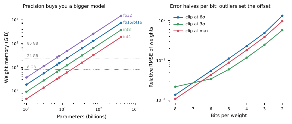
Figure 1:Precision is the lever that decides what runs on your hardware. Left: weight memory from the equation against model size, with three common VRAM limits marked; dropping from fp16 to 4 bits moves the largest feasible model up by roughly a factor of four. Right: a simulation of round-trip quantization error for Gaussian weights under uniform grids with three clipping rules. Relative error falls by about a factor of two per additional bit, and the choice of clipping threshold --- that is, how the rare large weights are handled --- sets the level of the whole curve.
:width: 90%
1.2Quantization as Deliberate Measurement Error
Quantizing a weight matrix replaces each entry with the nearest point on a coarse grid. For a symmetric uniform scheme with bits and scale ,
and the induced error behaves, to first order, like measurement error on the coefficients. The naive analysis --- treat as uniform on , note the variance is , conclude that error falls by a factor of two per bit --- is a useful first pass and is what the right panel of Figure the figure shows. It also explains why practice departs from it: is set by the largest weight in the group, so a handful of outlier weights inflates the step size for everything else. Every serious quantization method is a response to that fact, whether by grouping weights into small blocks with their own scales, keeping outlier channels in higher precision, or choosing the grid to be optimal for a normal prior, as in the NF4 format of QLoRA Dettmers et al., 2023. (The two post-training schemes you will meet by name when downloading weights, GPTQ Frantar et al., 2022 and AWQ Lin et al., 2023, are both of this kind: each uses a small calibration sample to decide which weights may be coarsened and which must be protected, which makes the calibration set a design choice worth recording.) It is tempting to push the measurement-error analogy one step further, to attenuation bias, and the intuition is partly right. In a linear model, mean-zero error in a covariate biases its coefficient toward zero, and one might expect mean-zero rounding of the weights to leave the output unchanged in expectation. It does not, and the reason is instructive: the weight error is not independent of the weight, because the scale is set by the largest entry in the group, so the quantization of a coefficient is correlated with the values of its neighbours, and the per-layer errors then pass through nonlinearities that do not preserve zero mean. That is enough to see that the output degradation is not a mean-zero perturbation and cannot be assumed to wash out. But the honest thing is to stop there. A deep network is not a linear model, the errors compound across dozens of layers in a way no closed form captures, and pushing the errors-in-variables picture past this single paragraph would claim a precision the analogy does not have. The value of the analogy is diagnostic --- it tells you the effect is real and structured, not that you can compute it.
Because the theory does not give a usable prediction, the discipline that matters is empirical, and it is one this readership already practises. Quantize the model, then measure two things: perplexity on a held-out corpus, which is a likelihood-based goodness check that is cheap and task-agnostic, and accuracy on your actual downstream task, which is the quantity you care about and which perplexity can fail to track. The pattern most practitioners report is that 8-bit quantization is nearly free, 4-bit is usually acceptable, and below 4 bits quality degrades sharply --- but this is folklore, an aggregate over models and tasks that need not hold for yours, and it is offered here as a starting expectation to be re-verified rather than a result to be relied on. The specific failure the two-measurement protocol guards against is a quantization that barely moves perplexity while collapsing accuracy on a narrow task, which happens precisely when the task depends on the rare capabilities that the outlier weights encoded.
1.3Adapting a Local Model Without Retraining It
Full fine-tuning of even a 7B model requires optimizer state several times the size of the weights and is out of reach for most local hardware. Low-rank adaptation sidesteps this by freezing and learning a low-rank update Hu et al., 2021,
which trains a fraction of a percent of the parameters and yields an adapter file of a few tens of megabytes. Combining a 4-bit frozen base with a low-rank update in higher precision --- QLoRA --- brings fine-tuning of a mid-sized model onto a single consumer GPU Dettmers et al., 2023. The statistical reading is that is a rank constraint acting as a regularizer, and the effective number of parameters, not the nominal one, governs how much data you need. The full treatment of parameter-efficient fine-tuning --- the optimization, the variants, the theory of why a low-rank update suffices --- belongs to the chapter on modern training, and the reader who wants it should go there. Here only the statistical reading and one piece of practical guidance are needed. The reading is that the rank in the equation is a rank constraint on the update, and a rank constraint is a regularizer: it fixes the effective number of new parameters, and it is that effective number, not the nominal parameter count of the base model, that governs how much adaptation data you need. The practical guidance is that between 8 and 64 covers most cases, and it is a knob to be chosen the way any regularization strength is chosen, by watching held-out behaviour. Too large an wastes parameters and can overfit a small adaptation set; too small an underfits, and the symptom is distinctive --- the adapted model behaves as though it never saw your instructions, because a rank too low to represent the change you asked for leaves the base model’s behaviour essentially intact. If a LoRA fine-tune seems to have done nothing, raising the rank is the first thing to try.
1.4A Reproducible Local Workflow
The reason to prefer a local model in a paper is that it can be pinned. Record the model repository and revision hash, the quantization format, the runtime and its version, the decoding parameters, and the seed --- all five, because any one of them can change your outputs. Even then, exact bitwise reproducibility across different GPUs or batch sizes is not guaranteed, so the honest claim is distributional reproducibility, and the honest report includes several seeds.
name, rev = “microsoft/Phi-4-mini-instruct”, “main” # pin a commit hash here tok = AutoTokenizer.from_pretrained(name, revision=rev) model = AutoModelForCausalLM.from_pretrained( name, revision=rev, torch_dtype=torch.bfloat16, device_map=“auto”)
msgs = [{“role”: “user”, “content”: “State Bayes’ theorem in one sentence.”}] ids = tok.apply_chat_template(msgs, add_generation_prompt=True, return_tensors=“pt”) torch.manual_seed(0) out = model.generate(ids.to(model.device), max_new_tokens=128, do_sample=True, temperature=0.7, top_p=0.95) print(tok.decode(out[0, ids.shape[-1]:], skip_special_tokens=True)) print(torch.cuda.max_memory_allocated() / 2**30, “GiB peak”)
Four runtime families cover essentially all local work, and it is worth naming them without endorsing one, because the right choice depends entirely on the job. Hugging Face transformers is the research default: it exposes logits and per-token log-probabilities, which the perplexity comparison of Exercise 5 requires and which a chat interface hides. llama.cpp, with its GGUF file format, targets CPU and Apple silicon and is the route when no GPU is available Gerganov & llama.cpp contributors, 2023. vLLM is built for batched throughput and is what an evaluation over thousands of prompts should use. And a range of point-and-click front ends exist for exploration, where the convenience is worth the loss of control. The one thing that traps new users is the file-format split: GGUF files load into llama.cpp and its wrappers but not into transformers, while safetensors checkpoints load into transformers but not into llama.cpp without a conversion step, and a converted file carries whatever quantization choices the converter made. Check that the weights you download are in the format your chosen runtime reads before assuming a failure to load is a deeper problem.
The primary sources are few. Adaptation under memory constraints is Hu et al. (2021) for low-rank adaptation and Dettmers et al. (2023) for its quantized form, which is what brings fine-tuning of a mid-sized model onto a single consumer GPU. The whole enterprise of trading numerical precision for memory descends from mixed-precision training Micikevicius et al., 2018, which established that a model could be trained and run in half precision without meaningful loss --- the ancestor of every quantization scheme in this section. At the opposite end of the scale, when a model is too large for any single device, the memory is partitioned across many by methods such as ZeRO Rajbhandari et al., 2020; the arithmetic is the same budget as the equation and the equation, distributed rather than reduced.
1.5Tools in Practice
The categories below are what stands between a file of weights and a number in your paper. They are worth learning as categories, because the products inside each one turn over quickly while the division of labour between them has been stable: something loads weights, something quantizes them, something serves them at throughput, and something records what you ran.
[Research-oriented model library] Load and inspect. Hugging Face
transformersand its ecosystem: load weights by repository and revision, get the tokenizer and chat template that belong to them, and reach logits directly. Fits: anything that needs per-token log-probabilities --- the perplexity comparison of Exercise 5 cannot be done through a chat interface. Watch: defaults are convenient and unpinned. Pass an explicit revision, an explicit dtype and an explicit seed, or the object you loaded today is not the object you load next year.[Quantized-file runtime] CPU and consumer-hardware execution.
llama.cppand the GGUF file format it defines run quantized models on CPU and on Apple silicon;Ollamawraps the same machinery behind a model-pull command and a local HTTP endpoint. Fits: laptop-scale work, and any setting where no GPU is available. Watch: the file-format split is the trap. GGUF files do not load intotransformersandsafetensorscheckpoints do not load intollama.cppwithout conversion, and a converted file inherits the quantization choices of whoever converted it.[Throughput-oriented serving engine] Batched inference. vLLM and similar servers keep a GPU busy across concurrent requests, principally by managing the key--value cache of the equation in fixed-size pages rather than per-request slabs Kwon et al., 2023. Fits: scoring thousands of prompts, which is what an evaluation actually is. Watch: batching changes reduction order, so results are not bit-identical to the unbatched run. Fix the batch size along with the seed, and report distributional rather than exact reproducibility.
[Post-training quantizers] Compression. GPTQ Frantar et al., 2022 and AWQ Lin et al., 2023 choose a coarse grid using a small calibration corpus, protecting the outlier weights that inflate the scale in the equation. Fits: the step between “the model does not fit” and “the model fits”. Watch: the calibration corpus is a design choice. A model calibrated on generic web text and deployed on clinical notes has been coarsened where it mattered; record which pre-quantized file you downloaded, not just the bit width.
[Parameter-efficient fine-tuning stacks] Adaptation. Libraries implementing the equation and its quantized variant, so that a rank- adapter can be trained on one consumer GPU Hu et al., 2021Dettmers et al., 2023. Fits: teaching a local model a house format or vocabulary without touching the base weights. Watch: an adapter is meaningless without its base model and revision. Ship both, or the few tens of megabytes you saved are unusable.
[Local embedding and reranking models] Retrieval components. The same open-weight route applies to the encoders of Section that section, which are small enough to run on CPU. Fits: keeping an entire retrieval pipeline inside your institution’s network, which is usually the reason the governance question arose in the first place. Watch: embeddings from different models are not comparable, so a change of encoder invalidates a stored index and every distance computed from it.
Before downloading anything, do the arithmetic. The calculation below combines the equation and the equation with a bandwidth-bound throughput ceiling; substitute your own device’s memory and bandwidth, which the runtime or the data sheet will tell you, and read off which configurations are feasible.
import numpy as np
GiB = 2**30
vram = 24.0                                  # your device, in GiB; read it from the runtime
bw = 400.0                                   # its memory bandwidth in GB/s, from the data sheet
N, L, Hkv, dh = 13e9, 40, 8, 128             # 13B-class, 8 key/value heads (grouped-query)
print(" w-bits  kv-bits  context   weights   KV cache   total+20%   fits   tok/s ceiling")
for bw_, kvb, T in [(16, 16, 8192), (8, 16, 8192), (4, 16, 8192),
                    (4, 16, 65536), (4, 8, 65536), (4, 8, 262144)]:
    w = N * bw_ / 8 / GiB
    kv = 2 * L * Hkv * dh * T * kvb / 8 / GiB
    tot = 1.20 * (w + kv)
    print(f"{bw_:7d}  {kvb:7d}  {T:7d}   {w:7.2f}   {kv:8.2f}   {tot:9.2f}   "
          f"{str(tot <= vram):>5s}   {bw / (w + kv):13.1f}")
Tstar = N * 16 / 8 / (2 * L * Hkv * dh * 16 / 8)
print(f"context at which the cache equals the fp16 weights: {Tstar:.0f} tokens")
print(f"same for 4-bit weights and fp16 cache:              {Tstar / 4:.0f} tokens")
w-bits kv-bits context weights KV cache total+20% fits tok/s ceiling
16 16 8192 24.21 1.25 30.56 False 15.7
8 16 8192 12.11 1.25 16.03 True 29.9
4 16 8192 6.05 1.25 8.76 True 54.8
4 16 65536 6.05 10.00 19.26 True 24.9
4 8 65536 6.05 5.00 13.26 True 36.2
4 8 262144 6.05 20.00 31.26 False 15.4
context at which the cache equals the fp16 weights: 158691 tokens
same for 4-bit weights and fp16 cache: 39673 tokensThe first row does not fit and the second does, which is the whole practical content of quantization. Two further readings are worth extracting. The throughput ceiling in the last column is bandwidth divided by bytes touched per token, and it falls as the context grows even though the weights have not changed: generation is memory-bound, so a longer conversation is slower for a reason that has nothing to do with arithmetic. And the crossover context --- where cache equals weights --- moves down by exactly the compression factor, so the more aggressively you quantize the weights, the sooner the cache becomes the binding constraint. That is why cache quantization and paged allocation Kwon et al., 2023 appear immediately after weight quantization in every serving stack: they are the next term in the same budget.
Substitute your own numbers before trusting any of this. The point of the calculation is that it is a calculation, not a benchmark: it takes two device constants and four model constants, all of which are published, and returns a feasibility answer that does not depend on anyone’s marketing.
1.6Exercises
Using the equation and the equation, compute the total memory needed to serve a 13B-parameter model (, , ) at
fp16weights andfp16cache with a 16{,}384-token context. At what context length does the cache exceed the weights?Show that for weights uniform on rounding error the mean squared error is , and hence that relative RMSE falls by a factor of two per additional bit. Then explain, in one paragraph, why the right panel of Figure the figure shows the max-clipping rule beating the rule at 8 bits but losing to it at 2 bits.
Count the trainable parameters in the equation for a weight matrix at , and express the result as a fraction of the full matrix. What rank would be needed to reach ?
Computational. Simulate the weight distribution of one layer as a heavy-tailed draw (say scaled to sd 0.02), quantize it with the equation at , and plot the relative RMSE for per-tensor scaling versus per-block scaling with blocks of 64. Quantify how much of the improvement from blocking is attributable to the tail.
Computational. Run a small instruct model locally at
fp16and again at 4 bits, on the same 50 prompts with the same seed. Report the mean per-token log-likelihood under each and the fraction of prompts where the two answers differ materially. Comment on whether the perplexity change would have predicted the task-level change.
- Kwon, W., Li, Z., Zhuang, S., Sheng, Y., Zheng, L., Yu, C. H., Gonzalez, J., Zhang, H., & Stoica, I. (2023). Efficient Memory Management for Large Language Model Serving with PagedAttention. Proceedings of the 29th Symposium on Operating Systems Principles, 611–626. 10.1145/3600006.3613165
- Dettmers, T., Pagnoni, A., Holtzman, A., & Zettlemoyer, L. (2023). QLoRA: Efficient Finetuning of Quantized LLMs.
- Frantar, E., Ashkboos, S., Hoefler, T., & Alistarh, D. (2022). GPTQ: Accurate Post-Training Quantization for Generative Pre-trained Transformers. arXiv Preprint arXiv:2210.17323.
- Lin, J., Tang, J., Tang, H., Yang, S., Chen, W.-M., Wang, W.-C., Xiao, G., Dang, X., Gan, C., & Han, S. (2023). AWQ: Activation-aware Weight Quantization for LLM Compression and Acceleration. arXiv Preprint arXiv:2306.00978.
- Hu, E. J., Shen, Y., Wallis, P., Allen-Zhu, Z., Li, Y., Wang, S., Wang, L., & Chen, W. (2021). LoRA: Low-Rank Adaptation of Large Language Models.
- Gerganov, G., & llama.cpp contributors. (2023). llama.cpp: LLM inference in C/C++. https://github.com/ggml-org/llama.cpp
- Micikevicius, P., Narang, S., Alben, J., & others. (2018). Mixed Precision Training.
- Rajbhandari, S., Rasley, J., Ruwase, O., & He, Y. (2020). ZeRO: Memory Optimizations Toward Training Trillion Parameter Models.