1Modern LLMs
The previous chapters built a language model out of parts a statistician already owns: a categorical conditional distribution, a chain-rule factorization, and maximum likelihood. What separates a modern large language model from that description is not a new estimator but three things layered on top of it --- an enormous corpus, a training budget chosen by an empirical scaling relationship, and a post-training stage that reshapes the predictive distribution toward outputs humans prefer. This section is about that stack, and about reading the claims made for it with the skepticism you would bring to any other fitted model. The vocabulary is unfamiliar, but the underlying questions are the ones you ask every day: what is the estimand, what is the sampling distribution of the reported number, what does the model extrapolate, and what is the training population. A statistician who can answer those four questions about an LLM understands the technology better than most of the people deploying it. The practical payoff is knowing which knobs --- context, decoding temperature, system prompt, model size --- actually change the predictive distribution and which merely change how you sample from it.
Table 1:A dictionary for modern large language models: almost every component is a familiar statistical object under a new name, and the entries in the last column are where the correspondence breaks down.
| ML / AI term | Statistical analogue | What is the same | What is different / the catch |
|---|---|---|---|
| Foundation model | A fitted model reused across studies; a population reference model | One expensive fit amortized over many downstream analyses | The “population” is a scraped corpus nobody characterized; there is no sampling frame |
| Pretraining | Maximum likelihood on a very large sample | Same objective: minimize mean negative log-likelihood | One pass over the data is typical, so the fit never reaches the MLE; early stopping is implicit |
| Scaling law | A power-law regression of loss on sample size and model size | Fitting a parametric curve and extrapolating | Extrapolation is often two orders of magnitude beyond the fitted range, usually without error bars |
| Compute-optimal training | Constrained optimization of a fitted loss surface | Allocating a fixed budget between two design factors | The constraint is an engineering approximation, not an identity |
| Emergent ability | A threshold effect in a dose--response curve | A sharp change in an outcome as a covariate increases | Often an artifact of a discontinuous metric (exact match); smooth metrics show smooth curves |
| Instruction tuning | Fitting on a curated subsample after a general fit | Supervised learning on labelled input--output pairs | Changes the model’s style far more than its knowledge; easy to mistake one for the other |
| RLHF / preference tuning | Fitting a Bradley--Terry model, then optimizing against it | Paired-comparison likelihood, exactly as in ranking studies | The reward model is an estimate; optimizing hard against it exploits its error (reward hacking) |
| Temperature | A tempered / annealed likelihood | Reweights a distribution toward or away from its mode | Changes only how you sample, never what the model believes |
| Context window | The conditioning set of a predictive distribution | Everything in it enters the conditional | Position within the window matters empirically; information in the middle is used less |
| Hallucination | Confident extrapolation outside the support of the data | A model asked to predict where it has no information | The output carries no standard error, so the extrapolation is invisible to the reader |
| Benchmark score | A point estimate on a finite test sample | A sample mean with binomial error | Reported without a CI, on a test set that may be in the training corpus (contamination) |
| Chat template | A fixed design matrix encoding roles | Structure imposed on the input before fitting | Getting it wrong silently degrades output; it is a per-model convention, not a standard |
| Tokens | The unit of observation in the likelihood | The thing being counted and predicted | Not words; token counts differ across languages, which makes per-token pricing and context limits unequal |
1.1What “Large” Bought Us
The architecture of a modern LLM is essentially the decoder half of the transformer introduced in Vaswani et al. (2017) and popularized for generative use by Radford et al. (2018), Radford et al. (2019). Nothing in that architecture predicts that scaling it up by four orders of magnitude would produce a system that writes usable code; that fact was discovered empirically Brown et al., 2020. For a statistician the interesting content is that the field found a reproducible regression relationship between resources and out-of-sample loss, and then used it as a design tool. It helps to organize the last decade into three dates, because they are three different kinds of advance. In 2017 the transformer architecture arrived Vaswani et al., 2017; in 2020 the field established that scaling that architecture across several orders of magnitude reliably improved out-of-sample loss and, at sufficient scale, produced few-shot competence Brown et al., 2020; and in 2022 a post-training stage aligned the resulting predictive distribution to human preferences and turned a next-token predictor into an assistant Ouyang et al., 2022. Of the three, only the last is a genuinely new statistical idea --- fitting a preference model and optimizing a policy against it, developed below. The architecture is an engineering advance in how a conditional distribution is parameterized, and the scaling result is, for a statistician, a regression: a fitted power law relating resources to loss. That middle advance is the one the reader is best equipped to critique, and this section spends most of its length doing so, because a regression used two decades outside its fitted range is exactly the kind of claim our training makes us suspicious of.
One thing should be said plainly and once: the reader will not train one of these models. Pretraining a frontier model costs more than most university departments spend in a decade, and nothing in this book is a recipe for doing it --- the chapter on language modelling already makes the case that the interesting statistical questions lie in using these models rather than fitting them. What the reader will actually do is run open-weight models on their own hardware, which Section that section develops, and ground a model’s outputs in a document collection they control, which is the subject of retrieval-augmented generation. The purpose of understanding the training stack is not to reproduce it; it is to read the claims made for it correctly, and to know which of the knobs exposed to a user actually change the model. The claim that “more data lowers the loss” has a precise form the reader can check on a model small enough to hold in the head. Here a five-state Markov chain plays the role of the corpus: the entropy rate of the true chain is the term in the equation, and the fitted transition table is a language model with 20 free parameters.
import numpy as np
rng = np.random.default_rng(0)
V = 5
P = rng.dirichlet(np.ones(V) * 0.4, size=V)          # true bigram transition matrix
pi = np.linalg.matrix_power(P, 500)[0]               # stationary distribution
H = -(pi[:, None] * P * np.log(P)).sum()             # entropy rate, nats/token

def draw(n):
    x = np.zeros(n, dtype=int)
    u = rng.random(n)
    cdf = P.cumsum(1)
    for t in range(1, n):
        x[t] = np.searchsorted(cdf[x[t - 1]], u[t])
    return x

test = draw(20000)
for n in [500, 5000, 50000]:
    tr = draw(n)
    C = np.zeros((V, V))
    np.add.at(C, (tr[:-1], tr[1:]), 1.0)
    Phat = (C + 1) / (C + 1).sum(1, keepdims=True)   # smoothed MLE
    ce = -np.log(Phat[test[:-1], test[1:]]).mean()
    print(f"n = {n:6d}   held-out cross-entropy = {ce:.4f}   excess over floor = {ce - H:+.4f}")
print(f"irreducible entropy rate E = {H:.4f} nats/token")
n = 500 held-out cross-entropy = 1.3601 excess over floor = +0.0258
n = 5000 held-out cross-entropy = 1.3364 excess over floor = +0.0022
n = 50000 held-out cross-entropy = 1.3355 excess over floor = +0.0013
irreducible entropy rate E = 1.3343 nats/tokenHeld-out cross-entropy falls toward the entropy rate and stops there. That floor is a property of the data-generating process, not of the estimator: no architecture and no budget crosses it, which is why appears as an additive constant in every published scaling law rather than as something to be optimized away.
1.2Scaling Laws as a Regression Problem
The empirical finding is that test cross-entropy is well described by a power law in parameter count and training tokens Kaplan et al., 2020Hoffmann et al., 2022,
where is the irreducible entropy of the text itself and the two remaining terms are the penalties for a finite model and a finite sample. This is a nonlinear regression with five parameters fitted to a few hundred training runs, and it should be read as such: the exponents are estimates, the additive form is an assumption, and the residual structure is rarely reported. If training compute is approximately , minimizing the equation subject to that constraint gives the compute-optimal allocation
so that with the commonly quoted both the model and the dataset should grow as roughly the square root of the budget. The practical consequence --- that the models of the early 2020s were badly undertrained relative to their size --- was a purely statistical discovery, made by fitting a curve. A scaling law is a nonlinear regression, so it has standard errors, and the useful exercise is to fit one and then ask it a question outside the fitted range. The 36 synthetic “training runs” below span from 107 to 109; the extrapolation is to , one decade beyond the largest.
import numpy as np
from scipy.optimize import curve_fit
rng = np.random.default_rng(0)
E, A, al, B, be = 1.69, 406.4, 0.34, 410.7, 0.28     # published Chinchilla constants
N = np.repeat(np.geomspace(1e7, 1e9, 6), 6)          # 36 training runs
D = np.tile(np.geomspace(1e9, 1e11, 6), 6)
L = (E + A / N**al + B / D**be) * np.exp(rng.normal(0, 0.01, N.size))

def f(ND, lE, lA, a, lB, b):
    n, d = ND
    return np.log(np.exp(lE) + np.exp(lA) / n**a + np.exp(lB) / d**b)

p, cov = curve_fit(f, (N, D), np.log(L), p0=[0.5, 6.0, 0.3, 6.0, 0.3], maxfev=20000)
se = np.sqrt(np.diag(cov))
print(f"alpha = {p[2]:.4f} (SE {se[2]:.4f})   truth {al}")
print(f"beta  = {p[4]:.4f} (SE {se[4]:.4f})   truth {be}")
g = (np.array([1e10]), np.array([1e11]))              # 10x beyond the largest fitted model
J = np.array([(f(g, *(p + 1e-6 * np.eye(5)[i]))[0] - f(g, *p)[0]) / 1e-6 for i in range(5)])
mid = np.exp(f(g, *p)[0])
lo, hi = np.exp(f(g, *p)[0] + np.array([-1.96, 1.96]) * np.sqrt(J @ cov @ J))
print(f"extrapolated loss at N=1e10, D=1e11: {mid:.4f}   95% CI [{lo:.4f}, {hi:.4f}]")
print(f"CI width = {hi - lo:.4f} nats, and that ignores all error in the functional form")
alpha = 0.3569 (SE 0.0157) truth 0.34
beta = 0.2941 (SE 0.0223) truth 0.28
extrapolated loss at N=1e10, D=1e11: 2.2111 95% CI [2.1754, 2.2475]
CI width = 0.0721 nats, and that ignores all error in the functional formThe exponents are recovered to about two significant figures, and the extrapolated loss carries a delta-method interval that is wider than the improvements typically claimed between model releases. That interval is also optimistic: it conditions on the additive functional form being correct, which is the assumption most likely to fail out of range.
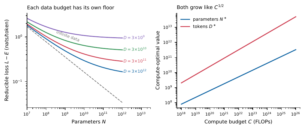
Figure 1:Reading a scaling law as a statistician reads a regression. Left: the fitted surface the equation evaluated at four data budgets; every finite corpus imposes a loss floor that no amount of additional capacity can cross, and only the infinite-data limit (dashed) is a clean power law. Right: the compute-optimal allocation the equation, which sends parameters and tokens up together rather than spending the whole budget on size. Constants are the published Chinchilla-style values; the point of the figure is the shape of the trade-off, not the specific numbers. :width: 90%
Equation the equation is derived by hand, but it can also be found numerically, which makes it easy to see what the constraint is doing. For each budget we grid over , set , and read off the minimizing pair.
import numpy as np
E, A, al, B, be = 1.69, 406.4, 0.34, 410.7, 0.28
Ngrid = np.geomspace(1e6, 1e13, 20001)
rows = []
for C in [1e18, 1e20, 1e22, 1e24]:
    D = C / (6 * Ngrid)                                # the constraint C = 6ND
    L = E + A / Ngrid**al + B / D**be
    i = L.argmin()
    rows.append((C, Ngrid[i], D[i]))
    print(f"C = {C:.0e}   N* = {Ngrid[i]:.3e}   D* = {D[i]:.3e}   tokens/param = {D[i]/Ngrid[i]:6.1f}   L = {L[i]:.4f}")
r = np.array(rows)
sN = np.polyfit(np.log(r[:, 0]), np.log(r[:, 1]), 1)[0]
print(f"fitted exponent of N* in C: {sN:.4f}   theory beta/(alpha+beta) = {be/(al+be):.4f}")
C = 1e+18 N* = 8.056e+07 D* = 2.069e+09 tokens/param = 25.7 L = 3.5353
C = 1e+20 N* = 6.448e+08 D* = 2.585e+10 tokens/param = 40.1 L = 2.5998
C = 1e+22 N* = 5.162e+09 D* = 3.229e+11 tokens/param = 62.6 L = 2.1386
C = 1e+24 N* = 4.129e+10 D* = 4.037e+12 tokens/param = 97.8 L = 1.9112
fitted exponent of N* in C: 0.4516 theory beta/(alpha+beta) = 0.4516The exponent recovered from the numerical optima matches to four decimals, confirming the algebra. The substantive output is the last column: the optimal tokens-per-parameter ratio is not a constant of nature but a slowly increasing function of the budget, which is precisely the point on which Chinchilla corrected its predecessors.
The critique a statistician should make of the equation is not that it is wrong but that it is used far outside where it was fitted. The exponents are estimated from runs spanning some range of and , and the resulting curve is then invoked to justify a training run one or two decades beyond the largest point in the fit. Extrapolation of a fitted regression that far past its support is exactly the operation every introductory course warns against, and the reason is not pedantry: the additive power-law form is an assumption about functional shape that the data inside the range cannot distinguish from several alternatives that diverge outside it. The honest way to report such an extrapolation is with a prediction interval that propagates both the parameter uncertainty and, ideally, the uncertainty in the functional form --- and the example above shows that even the parameter-only interval, computed by the delta method, is already wider than the loss improvements typically claimed between one model generation and the next. The telling fact is that essentially no scaling-law paper reports such an interval at all; the curve is drawn as if it were known, and the single extrapolated point is presented without the error bar that would let a reader judge it.
A related claim deserves the same scrutiny. “Emergence” is the assertion that a capability is absent at small scale and appears abruptly past some threshold. Before reading that as a discontinuity in the model, check what the metric is doing. Schaeffer et al. (2023) showed that many reported emergent abilities are artifacts of a discontinuous or nonlinear scoring rule: an exact-match metric is the product of per-token accuracies, and a product of smoothly improving factors can cross a visibility threshold sharply even though every underlying quantity is changing gradually. This is the familiar point that thresholding a smooth predictor manufactures a threshold effect --- the same mechanism that produces apparent dose thresholds in epidemiology when a continuous risk is dichotomized --- and it is why Wei et al. (2022), which catalogued the phenomenon, and its critique should be read together. The example below builds an “emergent” exact-match curve from a per-token accuracy that is smooth in log-scale, and it is worth noting in passing that a model whose per-token probabilities are well calibrated, in the sense of the calibration chapter, makes this decomposition exact rather than heuristic. “Emergence” is the claim that a capability appears abruptly at some scale. Before accepting it, check what the metric is doing: an exact-match score is the product of per-token accuracies, and a product of smooth increasing functions can look like a step.
import numpy as np
scale = np.geomspace(1e8, 1e12, 9)
per_token = 1 / (1 + np.exp(-(1.1 * np.log10(scale) - 12.4)))   # smooth in log-scale
exact = per_token**5                                            # 5 tokens must all be right
for s, a, e in zip(scale, per_token, exact):
    print(f"params = {s:8.1e}   per-token acc = {a:.3f}   exact-match acc = {e:.4f}")

def span(y):
    x = np.log10(scale)
    return np.interp(0.5, y, x) - np.interp(0.05, y, x)
print(f"decades of scale from 5% to 50%: per-token {span(per_token):.2f}, exact-match {span(exact):.2f}")
params = 1.0e+08 per-token acc = 0.027 exact-match acc = 0.0000
params = 3.2e+08 per-token acc = 0.045 exact-match acc = 0.0000
params = 1.0e+09 per-token acc = 0.076 exact-match acc = 0.0000
params = 3.2e+09 per-token acc = 0.125 exact-match acc = 0.0000
params = 1.0e+10 per-token acc = 0.198 exact-match acc = 0.0003
params = 3.2e+10 per-token acc = 0.299 exact-match acc = 0.0024
params = 1.0e+11 per-token acc = 0.426 exact-match acc = 0.0140
params = 3.2e+11 per-token acc = 0.562 exact-match acc = 0.0562
params = 1.0e+12 per-token acc = 0.690 exact-match acc = 0.1564
decades of scale from 5% to 50%: per-token 2.69, exact-match 0.57Per-token accuracy improves smoothly and takes 2.7 decades of scale to go from 5% to 50%; the exact-match score built from the very same numbers takes 0.6 decades and looks discontinuous. Nothing emerged. A statistician will recognize the mechanism as thresholding a smooth predictor, the same operation that manufactures apparent dose thresholds in epidemiology.
1.3The Post-Training Stack
A pretrained model predicts text; a deployed assistant answers questions. The bridge is post-training, usually a supervised instruction-tuning pass followed by preference optimization Ouyang et al., 2022Stiennon et al., 2020Ziegler et al., 2019. The preference stage is where the statistics are most familiar. Human annotators compare two candidate responses to a prompt and a reward model is fitted by the Bradley--Terry likelihood Bradley & Terry, 1952,
which is logistic regression on the difference of two learned scores. The policy is then tuned to maximize expected reward while staying close to the reference model,
a penalized objective in which the KL term plays exactly the role a prior plays in a penalized likelihood: it keeps the fit from chasing the noise in . Direct preference optimization Rafailov et al., 2023 shows that the equation has a closed-form solution that can be optimized directly from the pairwise data, collapsing the two-stage procedure into a single logistic-regression-like fit. The full derivation of the preference-optimization objective belongs to the chapter on modern training, and the reader who wants the policy-gradient machinery and the DPO reparameterization should go there; this section gives only the one-paragraph version and the statistical reading that matters most. That reading is this: reward hacking is overfitting to an estimated criterion. The reward model is not the thing anyone values; it is a Bradley--Terry fit to a finite sample of human comparisons, and like any fitted model it approximates the target with error. When the policy in the equation is optimized hard against , it does not learn to produce good responses --- it learns to produce responses that exploit wherever overestimates quality, which is precisely the region where the estimate is worst. This is the identical failure a statistician sees when a model is tuned against an estimated criterion rather than the truth: maximizing a proxy pushes the solution into the proxy’s error. The KL penalty is the guard, and it plays the role a penalty always plays, trading a little bias against a large reduction in the variance being chased; choosing its weight is the familiar problem of tuning a regularizer when the objective itself is noisy. The example below exhibits the effect with no policy gradient at all, by reweighting a population toward high estimated reward and watching the true reward peak and then fall. Equation the equation says a reward model is logistic regression on a difference of scores, and it can be fitted with an ordinary logistic routine by coding each comparison as a contrast vector with +1 for the winner and -1 for the loser. Watch both the recovered scores and what happens when the whole score vector is shifted.
import numpy as np
from sklearn.linear_model import LogisticRegression
rng = np.random.default_rng(0)
K, n = 6, 4000
r = np.array([0.0, 0.4, 0.9, 1.5, 1.8, 2.6])                    # true response quality
i, j = rng.integers(0, K, n), rng.integers(0, K, n)
keep = i != j
i, j = i[keep], j[keep]
win = rng.random(i.size) < 1 / (1 + np.exp(-(r[i] - r[j])))     # Bradley-Terry
X = np.zeros((i.size, K)); X[np.arange(i.size), i] = 1; X[np.arange(i.size), j] = -1
fit = LogisticRegression(fit_intercept=False, C=1e6, max_iter=1000).fit(X, win.astype(int))
rhat = fit.coef_[0]
print("true  r (centred):", np.round(r - r.mean(), 3))
print("fitted r (centred):", np.round(rhat - rhat.mean(), 3))
ll = lambda s: np.log(1 / (1 + np.exp(-np.where(win, 1, -1) * (s[i] - s[j])))).sum()
print(f"log-lik at rhat        = {ll(rhat):.6f}")
print(f"log-lik at rhat + 100  = {ll(rhat + 100):.6f}   (an additive shift is not identified)")
true r (centred): [-1.2 -0.8 -0.3 0.3 0.6 1.4]
fitted r (centred): [-1.205 -0.786 -0.26 0.23 0.575 1.446]
log-lik at rhat = -1768.472226
log-lik at rhat + 100 = -1768.472226 (an additive shift is not identified)The fitted rewards match the truth after centring, and the log-likelihood is exactly invariant to adding a constant to every score: the reward scale has no origin. This is the missing-intercept identifiability point of Exercise 3, and it matters in practice because a reward model’s absolute values are meaningless --- only differences are estimable, so a “reward of 3.5” reported without a reference is not a number.
Reward hacking is overfitting to an estimated criterion, and it can be shown without any policy gradient at all. Take a population of 5000 candidate responses, a true human value , and a fitted reward model that estimates with error; then reweight the population toward high estimated reward, with the KL penalty of the equation controlling how far the reweighting may go.
import numpy as np
rng = np.random.default_rng(0)
M = 5000
r_true = rng.normal(0, 1, M)                       # what humans actually value
r_hat = r_true + rng.normal(0, 2.0, M)             # the fitted reward model: an estimate
print(" lambda      KL   E_pi[r_hat]   E_pi[r_true]")
for lam in [np.inf, 4.0, 1.0, 0.5, 0.25, 0.1]:
    w = np.ones(M) / M if np.isinf(lam) else np.exp((r_hat - r_hat.max()) / lam)
    w = w / w.sum()
    wp = w[w > 0]
    print(f"{lam:7.2f}  {wp @ np.log(wp * M):6.3f}   {w @ r_hat:10.3f}   {w @ r_true:11.3f}")
print("proxy reward rises as the penalty is relaxed; true reward peaks and then falls")
lambda KL E_pi[r_hat] E_pi[r_true]
inf -0.000 0.030 -0.005
4.00 0.153 1.261 0.246
1.00 1.950 4.275 0.880
0.50 4.376 6.011 1.363
0.25 6.157 6.677 1.800
0.10 7.460 6.897 1.935
proxy reward rises as the penalty is relaxed; true reward peaks and then fallsThe proxy reward the optimizer sees rises monotonically as the penalty is relaxed, while the quantity anyone cares about peaks and then declines. The KL term is doing the job a penalty always does --- trading a little bias for a large reduction in the variance being chased --- and the tuning problem is the familiar one of choosing a penalty weight when the criterion itself is an estimate.
1.4Decoding: Sampling from a Predictive Distribution
Given the fitted conditional , generation is a sampling problem, and the knobs exposed by every API are reweightings of that distribution. Temperature scaling replaces the conditional by
so recovers greedy (modal) decoding and flattens toward uniform; top- and nucleus (top-) sampling instead truncate the conditional to its highest-probability set before renormalizing Holtzman et al., 2020. A related and widely used device is to condition the answer on an intermediate reasoning trace Wei et al., 2022, which changes the conditional the answer is drawn from without touching at all. None of these change the fitted model. (Every hosted API and every local runtime exposes , top- and top- under those names, so the same three knobs are in reach whether you call a provider endpoint or run weights on your own machine, for which see Section that section.) They change which summary of the predictive distribution you report, and a statistician should recognize the choice between a modal prediction and a draw as the same choice made between reporting a posterior mode and a posterior sample. Temperature and nucleus sampling are reweightings of a fixed conditional, so their effect can be read off a single next-token distribution without a model. The quantity to watch is the entropy, and the fact that the arg-max never moves.
import numpy as np
p = np.array([0.40, 0.22, 0.14, 0.09, 0.06, 0.04, 0.03, 0.02])   # a next-token distribution
ent = lambda q: -(q * np.log(q)).sum()
print("  tau   entropy(nats)   argmax   P(top-1)")
for tau in [0.2, 0.5, 1.0, 1.5, 2.0]:
    q = p**(1 / tau); q = q / q.sum()
    print(f"{tau:5.1f}   {ent(q):12.4f}   {q.argmax():6d}   {q.max():8.4f}")
for top_p in [0.9, 0.95]:
    keep = np.cumsum(p) <= top_p
    keep[np.argmax(np.cumsum(p) > top_p)] = True
    q = np.where(keep, p, 0.0); q = q / q.sum()
    print(f"top-p={top_p}: {keep.sum()} of {p.size} tokens kept, entropy {ent(q[q>0]):.4f}")
tau entropy(nats) argmax P(top-1)
0.2 0.2281 0 0.9467
0.5 1.0398 0 0.6595
1.0 1.6726 0 0.4000
1.5 1.8802 0 0.2986
2.0 1.9640 0 0.2495
top-p=0.9: 5 of 8 tokens kept, entropy 1.4006
top-p=0.95: 7 of 8 tokens kept, entropy 1.6067Temperature moves the entropy over an order of magnitude but never changes which token is most likely: is a monotone transformation of , so the mode is invariant. Top- truncation is a different operation --- it deletes mass rather than reweighting it --- and at it has already discarded three of eight candidate tokens, which is why combining aggressive truncation with high temperature does much less than it appears to.
This has a direct methodological consequence, and it is the most common analysis error in applied LLM papers. A model run at a nonzero temperature is a random number generator, yet a great many reported results are a single generation at whatever the default temperature happened to be, treated as though it were the deterministic output of the model. It is not. Two runs of the same prompt give different completions, and a conclusion drawn from one of them has an unreported run-to-run variance that can easily exceed the effect being claimed. The minimum defensible practice is to fix and report the decoding parameters --- temperature, top-, and the seed where the interface exposes one --- and to report results across at least five independent draws rather than one, so that the between-draw variability is visible and can be put into the standard error. This is nothing more than the elementary point about sampling variability that the chapter on inference makes for any stochastic procedure, applied to a stochastic procedure that is easy to mistake for a fixed function. A number obtained from a single generation at an unrecorded temperature is not reproducible and should not be reported as if it were.
1.5Reading Benchmark Claims
A benchmark number is a sample mean over a finite set of items, and the convention of reporting it without an interval would not survive review in any other field. If items are scored as correct or not, the binomial standard error is , so a 500-item benchmark resolves differences of roughly four percentage points and nothing finer. Two further problems have no clean analogue in ordinary practice: test items are frequently present in the training corpus (contamination), and the same public test sets are reused for years by thousands of groups, which is adaptive overfitting on a scale that makes the effective multiplicity impossible to count. (The pairwise “arena” leaderboards that increasingly supplement fixed benchmarks replace the binomial with the Bradley--Terry likelihood of the equation, fitted to votes from a self-selected user population Chiang et al., 2024; the estimand changes but the sampling problem does not.) A benchmark score is a binomial proportion, and contamination is the situation where some test items were memorized rather than solved. Both effects can be quantified in a few lines.
import numpy as np
rng = np.random.default_rng(0)
n, p_true = 500, 0.70
print(f"n=500, phat=0.80: 95% half-width = {1.96*np.sqrt(0.8*0.2/n):.4f}  (a 2-point gain is inside the noise)")
frac = 0.15                                                  # share of test items seen in training
mem = rng.random(n) < frac
correct = np.where(mem, 1, rng.random(n) < p_true)
phat = correct.mean()
se = np.sqrt(phat * (1 - phat) / n)
print(f"true ability = {p_true:.2f}, contaminated fraction = {frac:.2f}")
print(f"reported score = {phat:.4f}  95% CI [{phat - 1.96*se:.4f}, {phat + 1.96*se:.4f}]")
print(f"interval covers the true ability: {phat - 1.96*se <= p_true <= phat + 1.96*se}")
n=500, phat=0.80: 95% half-width = 0.0351 (a 2-point gain is inside the noise)
true ability = 0.70, contaminated fraction = 0.15
reported score = 0.7480 95% CI [0.7099, 0.7861]
interval covers the true ability: FalseThe reported score is biased upward by roughly the contaminated fraction times the headroom, and the nominal 95% interval --- correctly computed, from a correctly counted sample --- excludes the model’s true ability. This is the failure mode that makes benchmark leaderboards hard to read: the interval is honest about sampling error and silent about the bias, which is the larger of the two.
One worked number fixes the scale of the problem. At items and an observed accuracy of , the binomial standard error is , so the interval half-width is about 3.5 percentage points. A “state of the art” improvement of two points over the previous model is therefore comfortably inside the noise of a 500-item benchmark, and cannot be distinguished from no improvement at all without either a much larger test set or a paired analysis on identical items. The evaluation chapter’s section on benchmarks develops the full treatment --- the design-effect corrections, the multiplicity from reused test sets, the contamination adjustments --- and the reader should take the machinery from there; the point to carry out of this section is only that a benchmark number is a sample mean with a standard error, and a difference smaller than that standard error is not a result.
The primary sources for this section form a short reading list. The architecture is Vaswani et al. (2017); scale and few-shot prompting are Radford et al. (2019) and Brown et al. (2020); the scaling laws are Kaplan et al. (2020) and Hoffmann et al. (2022); instruction following is Ouyang et al. (2022); and the text-to-text framing that unified NLP tasks as sequence-to-sequence problems is Raffel et al. (2020). Of these, the reader who reads only one should read the Chinchilla paper Hoffmann et al., 2022, because it is itself a statistician’s move: a regression critique of an earlier regression, showing that the exponents in Kaplan et al. (2020) had been estimated in a way that misallocated the compute budget, and that a corrected fit implied the large models of the day were badly undertrained. It is the cleanest worked example in the literature of what careful attention to a fitted curve buys.
1.6Tools in Practice
The stack described above reaches a working statistician through a handful of tool categories, and the categories are considerably more stable than the products that occupy them. What follows is a map of those categories: the job each one does, the step of an analysis it belongs to, and the specific thing to check. Particular capabilities, interfaces and prices move fast enough that any snapshot printed here would be misleading within a year, so consult current documentation for specifics and take from this section only the frame in which to evaluate what you find.
[Hosted chat interface] Interactive front end. A browser or desktop client for one-off drafting, critique and exploration. Fits: the exploratory phase, before anything is scripted. Watch: nothing is pinned --- not the seed, not the decoding parameters, not the model revision --- so a number obtained here is not a number you can report.
[Provider API and SDK] Programmatic access. The same models reached from code, with the decoding parameters of the equation under your control and log-probabilities sometimes exposed. Fits: any analysis that must be re-runnable, which is every evaluation in this book. Watch: an endpoint name is not a version. Record whatever model identifier the response returns next to your results, and re-run the baseline when it changes.
[Batch or asynchronous endpoint] Offline scoring. Submit a file of prompts and collect the completions later, usually at reduced cost. Fits: scoring a fixed item set --- the loop in Exercise 5. Watch: completions return unordered and partial failures are quiet. Join on an item key you supplied and count the rows before you compute a proportion, or the denominator of your accuracy is wrong.
[Structured-output and tool-calling mode] Constrained decoding. Restrict generation to a caller-supplied JSON schema or function signature. Fits: turning free text into a data frame, which is most statistical use. Watch: the constraint is syntactic only. A schema-valid response can still report a number that appears nowhere in the source text.
[Pairwise arena and public leaderboard] Comparative evaluation. Aggregate human preferences between anonymized model pairs into a ranking Chiang et al., 2024. Fits: shortlisting two or three candidates before you run your own evaluation on your own task. Watch: the ranking is a fitted Bradley--Terry model over a self-selected voter population and an unspecified prompt distribution; adjacent entries are routinely inside each other’s estimation error, as the example below shows.
[Open-weight model hub] Distribution. A repository serving weights, tokenizer and revision hashes as downloadable artifacts. Fits: work that must be reproducible years from now, or that cannot leave your institution; Section that section develops this. Watch: a repository name without a revision hash is not a pinned object.
An agentic front end that runs a multi-step literature search and returns a long report with inline citations is a different instrument with a different failure surface, and it is treated separately in Section that section.
A leaderboard built from pairwise votes is a fitted model, so the difference between two entries has a sampling distribution. Simulate an arena with eight entrants whose true strengths are known and whose top two differ by 0.2 on the log-odds scale, then ask how many votes are needed before the ranking of those two is reliable.
import numpy as np
from sklearn.linear_model import LogisticRegression
rng = np.random.default_rng(0)
K = 8
theta = np.linspace(0.0, 1.4, K)                        # true Bradley-Terry strengths
gap = theta[-1] - theta[-2]

def arena(n_votes):                                     # one leaderboard from n_votes comparisons
    i, j = rng.integers(0, K, n_votes), rng.integers(0, K, n_votes)
    m = i != j
    i, j = i[m], j[m]
    win = rng.random(i.size) < 1 / (1 + np.exp(-(theta[i] - theta[j])))
    X = np.zeros((i.size, K)); X[np.arange(i.size), i] = 1; X[np.arange(i.size), j] = -1
    return LogisticRegression(fit_intercept=False, C=1e6, max_iter=2000).fit(
        X, win.astype(int)).coef_[0]

print(f"true gap between the top two entrants = {gap:.3f} log-odds")
print("  votes   SD of estimated gap   P(rank order of top two is correct)")
for n in [250, 1000, 4000, 16000]:
    fits = np.array([arena(n) for _ in range(150)])
    d = fits[:, -1] - fits[:, -2]
    print(f"{n:7d}   {d.std(ddof=1):18.3f}   {np.mean(d > 0):36.3f}")
true gap between the top two entrants = 0.200 log-odds
votes SD of estimated gap P(rank order of top two is correct)
250 0.441 0.660
1000 0.187 0.847
4000 0.087 0.980
16000 0.044 1.000At 250 votes the estimated gap is twice as variable as the gap itself and the leaderboard puts the better entrant on top only two times in three; several thousand votes are needed before the ordering is trustworthy. Public arenas do collect far more votes than this, but they also rank far more than eight entrants and the differences near the top are far smaller than 0.2, so the same arithmetic applies with the sign reversed. Read a leaderboard the way you would read any table of estimates without standard errors: the gross ordering is informative, adjacent rows are not, and the ranking answers a question about a voter population that is not your user population.
1.7Exercises
Fit the scaling form the equation to a small table of (parameters, tokens, loss) triples using nonlinear least squares. Report approximate standard errors for and , then form a prediction interval for the loss at a model ten times larger than the largest one in the fit. Comment on the width of that interval relative to the gains typically claimed for a new model.
Show that the compute-optimal allocation the equation follows from minimizing the equation subject to , and state precisely which step requires to be constant.
Verify that the equation is exactly a logistic regression with a single covariate, the score difference, and no intercept. What is the consequence of the missing intercept for the identifiability of ?
Computational. Take any next-token distribution --- from an API that returns log-probabilities, or from a small local model --- and plot the entropy of in the equation against for . Overlay the entropy after top- truncation at . Explain which combinations of the two knobs are redundant.
Computational. Score a model on 200 items of any small benchmark, five times with different seeds at temperature 1. Report the mean, the within-seed binomial interval, and the between-seed standard deviation. Which of the two sources of variability is larger, and which does the literature usually report?
- Vaswani, A., Shazeer, N., Parmar, N., Uszkoreit, J., Jones, L., Gomez, A. N., Kaiser, L., & Polosukhin, I. (2017). Attention Is All You Need.
- Radford, A., Narasimhan, K., Salimans, T., & Sutskever, I. (2018). Improving Language Understanding by Generative Pre-Training.
- Radford, A., Wu, J., Child, R., Luan, D., Amodei, D., & Sutskever, I. (2019). Language Models are Unsupervised Multitask Learners [Techreport]. OpenAI.
- Brown, T. B., Mann, B., Ryder, N., Subbiah, M., Kaplan, J., Dhariwal, P., Neelakantan, A., Shyam, P., Sastry, G., Askell, A., Agarwal, S., Herbert-Voss, A., Krueger, G., Henighan, T., Child, R., Ramesh, A., Ziegler, D. M., Wu, J., Winter, C., … Amodei, D. (2020). Language Models are Few-Shot Learners.
- Ouyang, L., Wu, J., Jiang, X., Almeida, D., Wainwright, C. L., Mishkin, P., Zhang, C., Agarwal, S., Slama, K., Ray, A., Schulman, J., Hilton, J., Kelton, F., Miller, L., Simens, M., Askell, A., Welinder, P., Christiano, P., Leike, J., & Lowe, R. (2022). Training language models to follow instructions with human feedback.
- Kaplan, J., McCandlish, S., Henighan, T., Brown, T. B., Chess, B., Child, R., Gray, S., Radford, A., Wu, J., & Amodei, D. (2020). Scaling Laws for Neural Language Models.
- Hoffmann, J., Borgeaud, S., Mensch, A., Buchatskaya, E., Cai, T., Rutherford, E., de Las Casas, D., Hendricks, L. A., Welbl, J., Clark, A., Hennigan, T., Noland, E., Millican, K., van den Driessche, G., Damoc, B., Guy, A., Osindero, S., Simonyan, K., Elsen, E., … Sifre, L. (2022). Training Compute-Optimal Large Language Models.
- Schaeffer, R., Miranda, B., & Koyejo, S. (2023). Are Emergent Abilities of Large Language Models a Mirage?
- Wei, J., Tay, Y., Bommasani, R., Raffel, C., Zoph, B., Borgeaud, S., Yogatama, D., Bosma, M., Zhou, D., Metzler, D., Chi, E. H., Hashimoto, T., Vinyals, O., Liang, P., Dean, J., & Fedus, W. (2022). Emergent Abilities of Large Language Models.
- Stiennon, N., Ouyang, L., Wu, J., Ziegler, D. M., Lowe, R., Voss, C., Radford, A., Amodei, D., & Christiano, P. (2020). Learning to summarize from human feedback.
- Ziegler, D. M., Stiennon, N., Wu, J., Brown, T. B., Radford, A., Amodei, D., Christiano, P., & Irving, G. (2019). Fine-Tuning Language Models from Human Preferences.
- Bradley, R. A., & Terry, M. E. (1952). Rank Analysis of Incomplete Block Designs: I. The Method of Paired Comparisons. Biometrika, 39(3/4), 324. 10.2307/2334029
- Rafailov, R., Sharma, A., Mitchell, E., Ermon, S., Manning, C. D., & Finn, C. (2023). Direct Preference Optimization: Your Language Model is Secretly a Reward Model.
- Holtzman, A., Buys, J., Du, L., Forbes, M., & Choi, Y. (2020). The Curious Case of Neural Text Degeneration.
- Wei, J., Wang, X., Schuurmans, D., Bosma, M., Ichter, B., Xia, F., Chi, E., Le, Q., & Zhou, D. (2022). Chain-of-Thought Prompting Elicits Reasoning in Large Language Models.