Everything in this chapter has described what these tools can do; this section describes the ways they fail, and argues that a statistician is unusually well placed to recognise those failures because each of them already has a name in our field. A fluent, confident, entirely fabricated citation is extrapolation beyond the support of the data, reported without a standard error. That failure is the one with a mechanical partial remedy --- every identifier in a reference list can be resolved against Crossref or the arXiv API, which settles existence but not support, a distinction developed in Section that section. A benchmark score that cannot be reproduced next month is an instrument recalibrated mid-study. A model that agrees with whatever framing you supplied is an interviewer effect. A capability number computed on material that was almost certainly in the training corpus is testing on the training data. Naming the failures this way is more than a rhetorical convenience, because it tells you which diagnostic to reach for and, more often, why the diagnostic you would ordinarily run cannot be run here: the sampling frame is undocumented, the training corpus is unreleased, and the space of prompts admits no natural grid over which to conduct a sensitivity analysis. Some of these gaps admit partial instrumentation --- a prompt-sweep runner such as promptfoo at least turns the last of them into a pre-specified sample rather than a single convenience draw --- and the tools that do so are collected at the end of this section. The catalogue in Table the concept table above is the map for the rest of this section, and it is also the list of caveats that belongs in the methods section of any paper whose analysis passed through a large language model.
Table 1:A dictionary for the failure modes of LLM-based tools: each one has a name a statistician already owns, and in every case the diagnostic that would catch it is harder to run here than in a regression.
| ML / AI term | Statistical analogue | What is the same | What is different / the catch |
|---|---|---|---|
| Hallucination, or confabulation | Extrapolation beyond the support of the training data, reported without a standard error | Both produce a confident answer in a region where the fit is supported by nothing, and in both cases the output looks exactly like the well-supported output | A regression at least warns you through a large leverage or a wide prediction interval. A language model emits fluent prose at identical confidence whether the claim is memorised, interpolated or invented, and fluency is not evidence |
| Model confidence, and self-reported certainty | A calibrated predictive probability | Both are numbers between zero and one attached to an assertion | Token-level likelihood measures the plausibility of the wording, not the truth of the claim, and instruction tuning degrades calibration further Guo et al. (2017), Minderer et al. (2021). Asking a model how sure it is elicits text about confidence, not a probability |
| Knowledge cutoff | A closed cohort with a fixed end of follow-up | Both mean that nothing after a certain date is in the data, so inference about later periods is extrapolation in time | The cutoff is approximate and porous: the corpus is not a clean cohort, coverage thins near the boundary, and retrieval or search tools mix in later material without any record of what came from where |
| Benchmark contamination | Testing on the training data; test-set leakage | Both inflate reported performance because the evaluation material was present during fitting Kaufman et al. (2012) | The training corpus is web-scale and usually undisclosed, so you cannot check. For a statistician this is the single most important caveat on every published capability number |
| Non-determinism at temperature above zero | Monte Carlo variability of a stochastic algorithm | Both mean that a repeated run gives a different answer, and both are handled by replication rather than by hoping | Seeds are often not exposed, and batching, hardware and silent model updates make results irreproducible even at temperature zero; a single run of an LLM-based analysis is a sample of size one from an unnamed distribution |
| Prompt sensitivity | Instability of a fit to an arbitrary analyst choice; researcher degrees of freedom | Both mean the conclusion depends on a decision that carries no scientific content, and both call for a sensitivity analysis over the choices | The space of prompts is unbounded and unstructured, so there is no natural grid to vary over and no accepted reporting standard for what was tried before the reported prompt was chosen |
| Sycophancy, and agreement with the user’s framing | Confirmation bias, and an interviewer effect in survey response | Both describe an instrument that returns what the questioner seems to want, which biases any conclusion drawn from it | It is induced by the preference tuning that made the model useful Ouyang et al. (2022), Bai et al. (2022), so it cannot be turned off; asking the model to check your work is asking a biased instrument to audit itself |
| Training-data bias and representational harm | Selection bias, and a convenience sample of unknown provenance | Both mean the fitted distribution reflects who and what was recorded rather than the population of interest Buolamwini & Gebru (2018), Mehrabi et al. (2021) | The sampling frame is undocumented and undocumentable at this scale, so there is no weight to apply and no way to characterise the target population Gebru et al. (2021) |
| Reasoning traces and chain-of-thought explanations | A post hoc rationalisation, not a derivation; a fitted explanation of an already-made prediction | Both are an account of how a conclusion was reached, produced after the machinery that reached it | The trace is generated text and need not correspond to the computation that produced the answer, so it is not an audit trail. This is the same faithfulness problem that afflicts post hoc interpretability generally Ribeiro et al. (2016), Lundberg & Lee (2017) |
| Context window and long-input degradation | A finite maximum lag, plus attenuation of information from the middle of a long record | Both impose a hard limit on how much material can influence a single answer | Retrieval fills the window with the material a retriever judged relevant, so what the model never sees is determined by a second fitted model whose errors are invisible in the output |
| Aggregate benchmark score | A single summary statistic reported for a heterogeneous population | Both compress performance across many cases into one number that is easy to compare | Averages hide subgroup failure, benchmarks are saturated and gameable, and the sample sizes behind headline differences are rarely large enough to support the ranking that gets published |
| Cost and latency per call | The computational budget of an analysis | Both constrain how many replicates, sensitivity runs or bootstrap resamples you can afford | Per-token pricing makes the honest workflow, repeating everything many times across prompts and seeds, the expensive one, so the incentive runs directly against the replication these tools most need |
| Data confidentiality when calling a hosted model | Disclosure risk, and the terms under which identifiable data may leave a study site | Both concern who is permitted to see the records, and both are governed by agreements rather than by technique | Sending protected records to a third-party endpoint is a disclosure, whatever the retention policy says; as noted for enterprise APIs above, this generally requires an institutional agreement or an open-weight model run locally |
| Silent model updates and version drift | A measurement instrument recalibrated mid-study without notification | Both break comparability between measurements taken at different times | An endpoint name is not a version. A result obtained today may not reproduce next month, which is why any published analysis using a hosted model must pin and report the exact version and date |
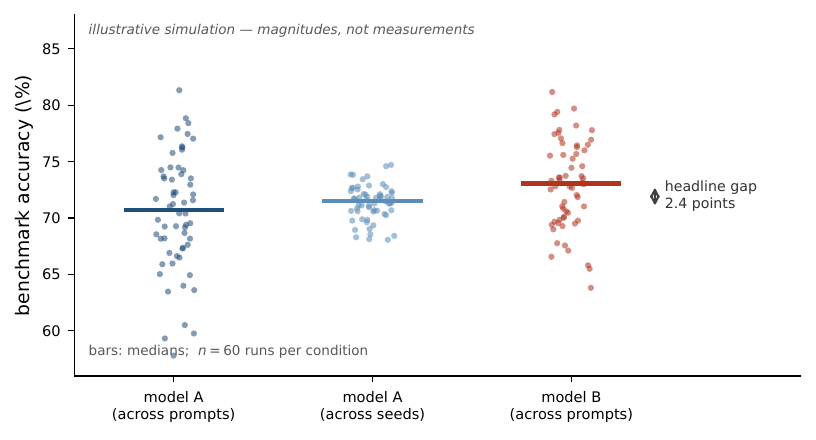
Figure 1:Why a single run of an LLM-based analysis is a sample of size one. Each point is one evaluation of the same benchmark; within a model, re-running under paraphrased prompts moves the score several times as much as re-running under a fresh random seed, and both spreads are larger than the 2.4-point gap between the two models’ medians that a paper would report as the result. The magnitudes here are illustrative rather than measured, but the ordering is the reproducible finding: nuisance variation from choices that carry no scientific content routinely exceeds the effect being claimed, which is why prompts, seeds, model versions and the number of repetitions belong in the methods section. :width: 90%
0.1Tools in practice
There is no tool that removes any row of Table the concept table above. What tooling can do is convert an unmeasured hazard into a measured one, and the useful way to read the following is as a list of instruments, each with its own sensitivity and specificity, attached to specific rows of that table. Three of the rows have partial mechanical remedies: fabricated references can be identifier-resolved, prompt sensitivity can be swept over a pre-specified family, and disclosure risk can be reduced by keeping the weights inside the institution. Three do not: contamination, sycophancy and the unfaithfulness of reasoning traces have no instrument that settles them, and a section that pretended otherwise would be doing the reader harm. For those, the honest move is the one a statistician already knows --- state the caveat in the methods section, bound what you can, and do not report a number whose provenance you cannot describe. A recurring failure pattern deserves naming in advance: every tool below is itself a fitted classifier or a heuristic, so each one has a false-negative rate, and a tool’s clean report is evidence about the tool as much as about the corpus.
[Crossref and arXiv resolvers] Reference verification. Public APIs that return a bibliographic record for a DOI or an arXiv identifier, so a reference list can be checked entry by entry. Fits: the hallucination row --- a census of non-existent citations before anything is submitted. Watch: resolution proves existence, not support; a real paper attached to a claim it does not make passes every automated check (Section that section).
[Microsoft Presidio] De-identification. Detects and redacts personal identifiers in free text using a combination of pattern rules, named-entity recognition and validation checksums. Fits: the confidentiality row --- reducing what leaves the study site when a hosted model is used. Watch: recall is well below one on realistic clinical prose, and a scrubber’s clean pass over a validation sample bounds the residual leak rate only as tightly as that sample is large, which the example below quantifies.
[Locally served open weights (Ollama, llama.cpp, vLLM)] Confidentiality and version control. Run a checkpoint you hold on hardware you control. Fits: the confidentiality row and the version-drift row simultaneously; nothing leaves, and nothing changes without your action. Watch: local weights remove the drift problem but not the others --- contamination, sycophancy and unfaithful reasoning traces are properties of the model, and they travel with the checkpoint.
[promptfoo] Prompt sensitivity sweeps. Runs a matrix of prompt variants against fixed cases and reports per-case outcomes. Fits: the prompt-sensitivity row --- it turns “we tried a few wordings” into a pre-specified family with recorded results. Watch: a sweep samples the prompt space, it does not integrate over it, so report the family you specified in advance and how it was chosen.
[Canary strings (the BIG-bench convention)] Contamination control. A unique identifier embedded in a benchmark file so that a model reproducing it demonstrates the file was in its training corpus. Fits: the contamination row, weakly --- it is a one-sided test. Watch: it detects only verbatim ingestion of documents that carried the canary; a negative result is close to uninformative, and no canary helps for benchmarks published before the convention existed.
[Guardrails-style output validators (Guardrails AI, NeMo Guardrails)] Output checking. Apply declarative checks --- schema conformance, banned content, groundedness against a source passage --- and block or retry on failure. Fits: the deployment seam, where an unchecked output would otherwise reach a user or a database. Watch: the validators are classifiers with their own error rates, and a retry-until-pass loop is a non-random filter on which inputs produce a recorded answer at all.
The confidentiality row is the one where a statistician's instinct pays off immediately, because the question "is this corpus safe to send" is a question about a rate and therefore about a sample size. The following runs a small pattern-based scrubber over eight synthetic notes with a known identifier count and then does the arithmetic that the audit implies. The notes and identifiers are invented for the example; the patterns are the kind that a rule-based de-identifier applies before any model is involved.
1Synthetic notes paired with the number of identifiers actually present.
notes = [(“Pt Ada Lovelace, MRN 4471902, seen 03/14/2021.”, 3), (“Discussed results with pt; nothing identifying here.”, 0), (“Contact daughter at 555-0142 regarding discharge.”, 1), (“Mr. O’Hara-Blake declined the biopsy on 7 Mar 2021.”, 2), (“MRN4471903 transferred from an outside hospital.”, 1), (“Follow-up in clinic in two weeks.”, 0), (“Pt Grace Hopper (mrn 4471904) tolerated the procedure.”, 2), (“Called 555 0143 twice; no answer.”, 1)]
patterns = [re.compile(r"\bMRN\s*\d{7}\b", re.I), # record number re.compile(r"\b\d{3}-\d{4}\b"), # phone re.compile(r"\b\d{2}/\d{2}/\d{4}\b"), # date re.compile(r"\b(?:Pt|Mr.|Mrs.|Ms.)\s+" r"[A-Z][a-z]+\s+[A-Z][a-z]+\b")]
found = [sum(len(p.findall(t)) for p in patterns) for t, _ in notes] truth = [k for _, k in notes] missed = [i for i, (f, k) in enumerate(zip(found, truth)) if f < k] print(f"identifiers present {sum(truth)} flagged {sum(found)}" f" recall {sum(found) / sum(truth):.2f}“) print(f"notes with a residual identifier: {missed}”)
2A clean validation sample is not a clean corpus.
for n_val in (20, 40, 100): hi = binomtest(0, n_val).proportion_ci(confidence_level=0.95, method=“exact”).high print(f"0 misses in {n_val:3d} audited -> rate <= {hi:.3f}" f" -> up to {round(20000 * hi):5d} leaks in 20,000 notes")
Two of the eight notes retain an identifier. A hyphenated surname, a date written as “7 Mar 2021” and a telephone number written with a space all defeat patterns that handle their more common forms, which is the characteristic error profile of a rule-based scrubber --- every flag it raised here is correct, and it misses on exactly the unusual formatting a production corpus is full of. The second block is the part worth carrying away. Suppose the audit had been clean. Zero misses in twenty audited notes bounds the miss rate above only by 0.168, which over a corpus of twenty thousand notes permits several thousand leaks; a hundred clean audits still permit several hundred. The rule of three is doing the work here --- with no observed events in trials the upper limit is about --- and it says that a clean sample is not a clean corpus. This is the same one-sided logic as the canary string above, and it is the reason the disclosure question is settled by an institutional agreement or by keeping the weights local, not by a scrubber’s clean report.
- Guo, C., Pleiss, G., Sun, Y., & Weinberger, K. Q. (2017). On Calibration of Modern Neural Networks. Proceedings of the 34th International Conference on Machine Learning (ICML), 1321–1330.
- Minderer, M., Djolonga, J., Romijnders, R., Hubis, F., Zhai, X., Houlsby, N., Tran, D., & Lucic, M. (2021). Revisiting the Calibration of Modern Neural Networks. Advances in Neural Information Processing Systems (NeurIPS), 34.
- Kaufman, S., Rosset, S., Perlich, C., & Stitelman, O. (2012). Leakage in Data Mining: Formulation, Detection, and Avoidance. ACM Transactions on Knowledge Discovery from Data, 6(4), 1–21. 10.1145/2382577.2382580
- Ouyang, L., Wu, J., Jiang, X., Almeida, D., Wainwright, C. L., Mishkin, P., Zhang, C., Agarwal, S., Slama, K., Ray, A., Schulman, J., Hilton, J., Kelton, F., Miller, L., Simens, M., Askell, A., Welinder, P., Christiano, P., Leike, J., & Lowe, R. (2022). Training language models to follow instructions with human feedback.
- Bai, Y., Jones, A., Ndousse, K., Askell, A., Chen, A., DasSarma, N., Drain, D., Fort, S., Ganguli, D., Henighan, T., Joseph, N., Kadavath, S., Kernion, J., Conerly, T., El-Showk, S., Elhage, N., Hatfield-Dodds, Z., Hernandez, D., Hume, T., … Kaplan, J. (2022). Training a Helpful and Harmless Assistant with Reinforcement Learning from Human Feedback.
- Buolamwini, J., & Gebru, T. (2018). Gender Shades: Intersectional Accuracy Disparities in Commercial Gender Classification. Proceedings of Machine Learning Research (FAT*), 77–91.
- Mehrabi, N., Morstatter, F., Saxena, N., Lerman, K., & Galstyan, A. (2021). A Survey on Bias and Fairness in Machine Learning.
- Gebru, T., Morgenstern, J., Vecchione, B., Vaughan, J. W., Wallach, H., III, H. D., & Crawford, K. (2021). Datasheets for Datasets.
- Ribeiro, M. T., Singh, S., & Guestrin, C. (2016). “Why Should I Trust You?”: Explaining the Predictions of Any Classifier.
- Lundberg, S., & Lee, S.-I. (2017). A Unified Approach to Interpreting Model Predictions.