import numpy as np
from scipy import stats

for n, correct in [(20, 17), (100, 85), (1000, 850)]:
    p = correct / n
    lo, hi = stats.beta.ppf([0.025, 0.975], correct + 0.5, n - correct + 0.5)  # Jeffreys
    print(f"n={n:>5}  accuracy={p:.3f}  95% CI=({lo:.3f}, {hi:.3f})  width={hi-lo:.3f}")
print("\nSame 85% at n=20 and n=1000 are not the same claim.")
n= 20 accuracy=0.850 95% CI=(0.651, 0.956) width=0.304
n= 100 accuracy=0.850 95% CI=(0.770, 0.910) width=0.139
n= 1000 accuracy=0.850 95% CI=(0.827, 0.871) width=0.044
Same 85% at n=20 and n=1000 are not the same claim.import numpy as np
from scipy import stats
rng = np.random.default_rng(6)
n = 200
difficulty = rng.normal(size=n) # item effect, shared by both prompts
a = (rng.normal(size=n) + 0.9 * difficulty + 0.25) > 0
b = (rng.normal(size=n) + 0.9 * difficulty) > 0
# Unpaired two-proportion test throws away the item pairing.
pooled = (a.sum() + b.sum()) / (2 * n)
se = np.sqrt(2 * pooled * (1 - pooled) / n)
z = (a.mean() - b.mean()) / se
print(f"prompt A={a.mean():.3f} prompt B={b.mean():.3f} diff={a.mean()-b.mean():+.3f}")
print(f"unpaired z={z:.2f} p={2*(1-stats.norm.cdf(abs(z))):.4f}")
# McNemar uses only the discordant pairs, which is where the information is.
n01 = int((~a & b).sum()); n10 = int((a & ~b).sum())
p_mc = stats.binomtest(n10, n10 + n01, 0.5).pvalue
print(f"discordant: A-only={n10}, B-only={n01} McNemar p={p_mc:.4f}")prompt A=0.575 prompt B=0.510 diff=+0.065
unpaired z=1.30 p=0.1920
discordant: A-only=41, B-only=28 McNemar p=0.1480import numpy as np
rng = np.random.default_rng(7)
# Two raters (say a human and a model) scoring 150 items pass/fail.
n = 150
truth = rng.random(n) < 0.6
human = np.where(rng.random(n) < 0.9, truth, ~truth)
model = np.where(rng.random(n) < 0.8, truth, ~truth)
obs = (human == model).mean()
p_h, p_m = human.mean(), model.mean()
exp = p_h * p_m + (1 - p_h) * (1 - p_m)
kappa = (obs - exp) / (1 - exp)
print(f"raw agreement = {obs:.3f}")
print(f"chance agreement = {exp:.3f}")
print(f"Cohen's kappa = {kappa:.3f}")
print("\nRaw agreement flatters a judge on imbalanced data; kappa does not.")raw agreement = 0.747
chance agreement = 0.526
Cohen's kappa = 0.466
Raw agreement flatters a judge on imbalanced data; kappa does not.1Evaluating LLM Outputs
Nothing in machine learning is more obviously a statistics problem, and more routinely done without statistics, than evaluating a language model. The prevailing practice is to run two systems on a benchmark, report two accuracies to three decimal places, and declare the larger one better. A statistician sees immediately what is missing: a standard error, a unit of analysis, a paired design, an adjustment for the dozens of comparisons already made on the same items, and any acknowledgement that the benchmark is a sample from a population of tasks nobody has defined. This section supplies that missing apparatus. We treat an evaluation as a designed experiment on a finite item pool: we compute the standard error of a benchmark accuracy, show why paired designs and McNemar’s test are the right default for comparing two systems on the same items, work out the sample size needed to detect the small gaps that actually separate modern systems, and confront the two structural problems that no amount of inference repairs --- test-set contamination, and using a language model as the judge of language models.
Table 1:Benchmark evaluation, translated: every element of a leaderboard has an exact counterpart in experimental design and diagnostic-test evaluation.
| ML / AI term | Statistical analogue | What is the same | What is different / the catch |
|---|---|---|---|
| Benchmark accuracy | A proportion estimated from a finite sample | Both need a standard error; both are useless without one | Benchmarks are reported without intervals, and items are neither a random sample from nor representative of any defined task population |
| Leaderboard ranking | Multiple comparisons on a shared test set | Both compare many candidates against common data | The test set is reused thousands of times, so the leader is partly selected on noise --- a winner’s curse with no correction applied |
| Head-to-head system comparison | Paired design on the same experimental units | Pairing removes item difficulty from the comparison | Almost all reported comparisons discard the pairing by quoting two marginal accuracies, wasting most of the available power |
| LLM-as-judge | A surrogate endpoint or a proxy rater | Both substitute a cheap measurement for an expensive one | The judge shares training data and failure modes with the systems it grades, so its errors are correlated with what it is grading Zheng et al., 2023 |
| Human preference win-rate | Bradley--Terry / Plackett--Luce paired comparison | Both estimate a latent quality scale from wins | Judges vary, drift, and reward fluency; the scale is preference, not correctness Bradley & Terry, 1952Plackett, 1975 |
| Test-set contamination | Training on the test set; information leakage | Both inflate apparent performance without improving the model | Contamination is undetectable from the outside for closed corpora, and it is near-certain for any public benchmark older than the model Kaufman et al., 2012 |
| Pass@ | Probability at least one of draws succeeds | An order statistic: under independence | Draws are correlated, so pass@ overstates what independent retries would give, and is often chosen after seeing the results |
| Automatic metric (BLEU, ROUGE) | A surrogate endpoint validated against a clinical one | Both are cheap proxies whose value rests on correlation with the real outcome | Correlation is weak at the individual-item level and vanishes once the metric is optimised against Papineni et al., 2002 |
| Model confidence / logprob | A predicted probability requiring calibration | Both are only interpretable when | Neural models are systematically overconfident, and instruction tuning can make calibration worse Guo et al., 2017 |
| Held-out evaluation split | An independent test sample | Both estimate out-of-sample performance | “Held out” from your fine-tuning is not held out from pretraining, which is the part you cannot inspect |
| Aggregate benchmark score | A composite endpoint | Both compress many outcomes into one number for ranking | The weights are implicit and arbitrary, and subgroup or task-level reversals are hidden by the aggregate |
1.1An accuracy is an estimate, so give it an interval
If a system answers evaluation items and are correct, the natural estimate is , with the Wilson interval Wilson, 1927 as the sensible default. The first thing this buys is calibration of expectations about resolution: at , the standard error of an accuracy near 0.8 is about 1.8 percentage points, so the difference between and on a 500-item benchmark is noise. The second thing it buys is the correct unit of analysis. If items are clustered --- several questions drawn from one document, several instances of one template --- then independence fails and the naive standard error is too small by a design-effect factor for clusters of average size and intra-cluster correlation . Benchmarks constructed by templating a handful of source documents are exactly this case. (Harnesses such as lm-evaluation-harness and HELM standardise how items are prompted and scored, which removes one source of between-paper incomparability, but they report the naive binomial interval and know nothing about your item clustering.) The calculation is worth doing on a realistic benchmark structure, because the correction is large and almost never applied. Take a benchmark of items built as 50 source templates with 20 instantiations each. Treated as independent items, an accuracy of 0.75 has a half-width of 2.7 percentage points. But items from one template share vocabulary, structure and difficulty, so they are correlated, and at an intra-cluster correlation of even the design effect is : the effective sample size collapses from to about 345, and the honest half-width widens to 4.6 points. At the effective sample size is 149 and the half-width is 6.9 points, more than double the naive figure.
import numpy as np

G, m, phat = 50, 20, 0.75            # 50 templates, 20 instantiations each
n = G * m
se_naive = np.sqrt(phat * (1 - phat) / n)
print(f"items n = {n},  accuracy = {phat},  naive 95% half-width = "
      f"{100 * 1.96 * se_naive:.1f} points")
print("rho   design effect   effective n   clustered 95% half-width   ratio")
for rho in (0.1, 0.2, 0.3):
    deff = 1 + (m - 1) * rho
    hw = 100 * 1.96 * se_naive * np.sqrt(deff)
    print(f"{rho:.1f}   {deff:12.1f}   {n / deff:11.0f}   {hw:22.1f}   "
          f"{np.sqrt(deff):.2f}x")
items n = 1000, accuracy = 0.75, naive 95% half-width = 2.7 points
rho design effect effective n clustered 95% half-width ratio
0.1 2.9 345 4.6 1.70x
0.2 4.8 208 5.9 2.19x
0.3 6.7 149 6.9 2.59xThe interval widens by a factor of roughly 1.7 to 2.6 across this plausible range of , which is the cheapest technical contribution a statistician can make to an ML evaluation paper and one essentially never made. The correct move is to estimate from the per-item outcomes --- a one-way random-effects fit clustered on the template --- and report the interval at the template level, or, more simply, to report accuracy per template and treat the 50 template means as the unit of analysis.
1.2Compare systems on the same items, and use the pairing
Two systems evaluated on the same items give a table of concordant and discordant results, with counts , , and . The difference in accuracy is and depends only on the discordant pairs; the concordant cells cancel. McNemar’s test McNemar, 1947 conditions on the number of discordant pairs and asks whether is binomial ,
where is the discordance rate. The variance of the paired difference depends on , and is small when two systems agree on most items --- which is precisely the situation when comparing two strong models. That is the statistical reason a paired design is not a refinement but a necessity here: it converts a comparison of two numbers near 0.8, each with a variance of about , into a comparison driven by a discordance rate that may be 0.05.
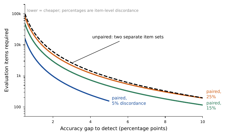
Figure 1:Detecting the small gaps that separate modern systems requires evaluation sets far larger than those in common use, and the paired design is what makes it affordable: detecting a two-percentage-point gap at power needs roughly items when the two systems disagree on of items, against about per arm for an unpaired comparison at baseline accuracy. Curves solve the equation at . :width: 90%
Sample size follows directly. To detect a true difference with power at level in a paired design,
which for and gives roughly items. Most published benchmarks are an order of magnitude smaller than that, which means most reported one- and two-point improvements are not distinguishable from noise by the very data used to claim them. Put plainly: the field’s evaluation sets are underpowered for the differences it routinely reports. A benchmark of a few hundred items cannot resolve a one- or two-point gap, and yet one- and two-point gaps are the currency of the leaderboard. The constructive remedy is not to make bigger claims but to make smaller ones honestly --- to report wider intervals computed at the correct unit of analysis, and to pre-register the effect size that would count as a real improvement before running the comparison, so that the analysis is not tuned to whatever gap happened to appear. Pre-registering the effect of interest also disciplines the sample size: the equation then tells you how many items the comparison needs, and a study that cannot afford them should say so rather than report an underpowered result as if it were decisive.
Reframing the question often helps more than more data. Much of the time the honest question is not “is model A better than model B?” but “is the cheaper model no worse than the expensive one by more than a tolerance I care about?” --- for instance, “is the small local model non-inferior to the hosted one by more than one point of accuracy?” That is an equivalence or non-inferiority question, and it is answered by two one-sided tests (TOST), not by a superiority test. In the TOST framing you specify a margin and reject the hypothesis of a meaningful difference only if the whole confidence interval for the paired difference lies within (for equivalence) or above (for non-inferiority). This inverts the burden of proof in the direction the deployment decision actually needs: a non-significant superiority test is not evidence of equivalence, whereas a TOST that rejects is. For choosing between models that are close in quality but far apart in cost, the TOST is very often the test the statistician should reach for, and it is essentially absent from the evaluation literature.
1.3The leaderboard is a multiple-comparisons problem
A public benchmark is a fixed test set queried by thousands of research groups, each choosing what to publish based on the result. This is adaptive data analysis and the consequence is a leader partly selected on noise: the expected accuracy of the maximum of noisy estimates exceeds the true best by roughly , so the top of a crowded leaderboard is optimistically biased by an amount that grows with participation. The statistical remedies are familiar --- a held-out set the submitters cannot query, a reusable-holdout mechanism that answers queries with calibrated noise Dwork et al., 2015, selection-adjusted intervals, or a hierarchical model shrinking each system toward the field mean --- and they are almost never applied. The magnitude is worth working out. Suppose groups submit to a leaderboard, each system’s accuracy is estimated with a standard deviation of percentage points, and --- the null worth considering --- all systems are in truth equally good. The reported leader is then the maximum of noisy estimates of a common mean, and the expected value of that maximum exceeds the truth by an amount that grows with . The extreme-value approximation gives , about 4.9 points at ; the exact expected optimism is a little smaller, and the example below puts it near 4 points by simulation. Either way the number is larger than the gaps leaderboards are used to adjudicate: the top-reported accuracy is optimistically biased by several points purely from selecting the maximum, before any real difference in ability enters.
import numpy as np

rng = np.random.default_rng(0)
sigma = 0.015                              # 1.5 points of estimation noise per system
print("K      sqrt(2 ln K) * sigma   Monte Carlo E[max]   (points of optimism)")
for K in (50, 200, 1000):
    approx = sigma * np.sqrt(2 * np.log(K))
    mc = (sigma * rng.standard_normal((200000, K)).max(1)).mean()
    print(f"{K:5d}   {100 * approx:18.2f}   {100 * mc:17.2f}")
K sqrt(2 ln K) * sigma Monte Carlo E[max] (points of optimism)
50 4.20 3.37
200 4.88 4.12
1000 5.58 4.86This is the winner’s curse, and it is the same phenomenon that inflates the estimated effect of the top-ranked gene in a genome-wide scan or the best-performing strategy in a backtest: the act of selecting the maximum biases the selected estimate upward, and a naive interval around it does not cover. The correct treatments are the tools of post-selection inference --- a held-out set the submitters cannot query, selection-adjusted intervals, or a hierarchical model that shrinks each system toward the field mean and reports the shrunken estimate. The benchmarks section of the evaluation chapter develops these at length; the point here is only that the leader of a crowded leaderboard is a selected estimate and must be read as one.
Contamination is the second structural problem, and it interacts with the first because it also biases the estimate upward in a way no interval captures. If a benchmark’s items were published before a model’s training cut-off, they may sit in its pretraining corpus, and the model may recall an answer it memorized rather than solve the item. This is the leakage problem of Kaufman et al. (2012) --- the same failure as training on the test set --- reappearing through the pretraining corpus, which is exactly the part of the pipeline an external evaluator cannot inspect. It is near-certain for any public benchmark older than the model. The practical detection heuristics all exist and are all weak, and the honest thing is to say so. Canary strings --- unique markers embedded in a benchmark so their later appearance signals ingestion --- only work if the benchmark authors planted them and the model provider did not filter them out. Memorization probes, which ask the model to complete a held-back portion of a known item, catch verbatim memorization but miss a model that memorized the answer without the surrounding text. A performance gap between items published before and after the training cut-off is suggestive but confounded with any genuine change in item difficulty over time. None of these gives a clean correction, so the defensible practice is to prefer benchmarks constructed after the model’s cut-off, to report the cut-off date alongside the score, and to treat any number from an old public benchmark as an upper bound on true ability.
1.4LLM-as-judge: a surrogate rater whose errors are correlated
Grading free-text output by hand does not scale, so the field grades it with another language model. Formally the judge is a diagnostic test for the event “the response is correct”, and its usefulness depends on sensitivity and specificity estimated against human labels. The trap is that the judge is not a random measuring device. It shares pretraining data, tokenisation and stylistic preferences with the systems it grades, so its errors correlate with theirs --- in particular it favours longer, more fluent, more confident answers, and it favours output from models like itself. Judge harnesses --- among them RAGAS for retrieval pipelines and the judge templates shipped with DeepEval and promptfoo --- make this measurement cheap to run and correspondingly easy to run without ever estimating and against human labels. Writing the judged accuracy in terms of the truth, ```{math}
:label: eq:evalllm-judge
\Pr(\text{judge says correct}) ;=;
p,\mathrm{se}_J ;+; (1-p),(1-\mathrm{sp}_J) ,
The primary sources for this section trace four threads. Automatic metrics and the practice of validating a cheap proxy against a costly ground truth begin with BLEU [@papineni2002bleu], whose limitations set the agenda for everything after it. The modern preference-based paradigm, in which quality is estimated from human pairwise comparisons rather than a reference answer, runs through @christiano2017deep, @stiennon2020learning, and @ouyang2022training. The requirement that a probability forecast be scored by a rule that rewards honesty --- so that a judge or a model cannot game the metric by misreporting its confidence --- is the theory of proper scoring rules [@gneiting2007strictly; @brier1950verification]. And the tradition of assessing whether stated probabilities match observed frequencies, which underlies both calibration and the reliability diagram, goes back to @dawid1982well and @degroot1983comparison. A reader assembling an evaluation methodology from scratch could do worse than to read one paper from each thread.

### Reporting: what a defensible evaluation table contains

The recommendation the book should make is short enough to fit in a paragraph. Report $n$ and how items were selected. Report accuracy with an interval computed at the correct unit of analysis. For comparisons, report the discordance table and a paired test rather than two marginal numbers. Report seed-to-seed and call-to-call variability alongside the item-level interval. State the model snapshot and decoding settings. Where a judge model was used, report its measured sensitivity and specificity on a human-labelled subsample and the size of that subsample. Report the scoring function itself, including any answer normalisation, since the example below shows it can reverse the ranking. None of this is novel statistics; all of it is missing from the typical results table.

### Tools in practice

Evaluation tooling divides into three jobs that are worth keeping separate in your head, because conflating them is how underpowered comparisons get published. A *harness* runs a fixed item set through a system under standardised prompting and scoring: its contribution is comparability, not inference. A *judge framework* replaces a human grader with a model, which is the surrogate-endpoint problem of [the equation](#eq:evalllm-judge) and is only interpretable with a human-labelled subsample attached. A *regression-test harness* asks a much narrower question --- did anything change since the last commit --- and it is the tool most researchers actually need and least often use. None of the three computes a paired test, a design effect, or a power calculation; those remain the statistician's contribution, and they are what this section supplies. The market here turns over quickly and specific feature claims date fast, so evaluate a candidate on durable properties: does it record per-item outcomes rather than only aggregates, can it re-score a stored run without re-querying the model, and does it let you attach the item's cluster identifier?

- [**lm-evaluation-harness**] *Benchmark harness.* Runs a large library of academic task definitions against local or hosted models with fixed prompting and scoring conventions. **Fits:** reproducing a published number, or placing your own model on the same footing as the literature. **Watch:** it reports aggregate accuracy with a naive interval; export the per-item results and do the inference yourself, especially when items are clustered by template.
- [**HELM**] *Multi-metric evaluation.* Evaluates a system across many scenarios and reports several metrics per scenario rather than one composite. **Fits:** the argument against a single aggregate score; it makes task-level reversals visible. **Watch:** more metrics is more comparisons, so a system that leads on one of many metrics has been selected on noise unless the selection is accounted for.
- [**Inspect**] *Evaluation framework.* A scripting framework for building custom evaluations with explicit datasets, solvers and scorers, with per-sample logs retained. **Fits:** domain evaluations you build yourself, which for most statistical applications is the only kind that measures the thing you care about. **Watch:** a bespoke evaluation is a bespoke instrument; report how items were selected, because a hand-built item set is a convenience sample.
- [**RAGAS**] *Retrieval-pipeline evaluation.* Scores a retrieval system on faithfulness of the answer to retrieved context and on the relevance of what was retrieved, mostly using a model as judge. **Fits:** separating retrieval failures from generation failures, which the end-to-end accuracy conflates. **Watch:** the scores are judge outputs, so they inherit [the equation](#eq:evalllm-judge) in full and need a human-labelled subsample before any of them can be read as a probability; for the harder case of a long generated report with inline citations, see Section [that section](tools_deep_research.md).
- [**DeepEval / promptfoo**] *Regression testing.* Run a fixed suite of assertions over prompts on every change and report which cases flipped. **Fits:** continuous monitoring of a deployed pipeline; the paired, per-item structure they store is exactly the discordance table [the equation](#eq:evalllm-mcnemar) needs. **Watch:** a suite that is re-run after every prompt edit becomes the thing being optimised, so hold out a set that is never used to make a change.
- [**Chatbot Arena--style pairwise collection**] *Preference data.* Collects human pairwise preferences and fits a latent quality scale from the wins. **Fits:** judging free-text quality where no reference answer exists; the model is Bradley--Terry [@bradley1952rank; @plackett1975analysis]. **Watch:** the estimand is preference, not correctness, the rater pool is self-selected and non-stationary, and prompt distribution drifts over time, so scales from different periods are not comparable.

<!-- TOY EXAMPLE: evalllm-tools-1 --> Before comparing systems it is worth measuring the measuring device, because the scoring function is an analysis choice with the same status as any other. Here two systems answer the same fourteen short-answer items; system B is more verbose but not less accurate. Scoring exactly and scoring after a trivial normalisation give two different discordance tables, and the paired test is run on both.

gold = ["hypertension", "42", "no", "chi-squared test", "1998", "type 2 diabetes", "0.05", "yes", "logistic regression", "three", "Bonferroni", "false", "n = 120", "left ventricle"] # Responses of two systems on the same 14 items, replayed from a stored log. sys_a = ["hypertension", "42", "no", "t-test", "1998", "type 1 diabetes", "0.05", "yes", "linear regression", "three", "Bonferroni", "true", "n = 120", "right ventricle"] sys_b = ["The answer is hypertension.", "42", "No.", "the chi-squared test", "1998", "Type 2 diabetes", "p = 0.05", "Yes", "logistic regression.", "Three", "The answer is Bonferroni.", "false", "n = 120", "the left ventricle"]

def exact(resp, ref): return resp == ref

_lead = re.compile(r"^(the answer is|answer:|the)\s+", re.I) def normalised(resp, ref): def norm(s): s = _lead.sub("", s.strip().lower().rstrip(".")) return re.sub(r"\s+", " ", s) return norm(resp) == norm(ref)

for label, score in (("exact match", exact), ("normalised ", normalised)): a = [score(r, g) for r, g in zip(sys_a, gold)] b = [score(r, g) for r, g in zip(sys_b, gold)] n10 = sum(x and not y for x, y in zip(a, b)) n01 = sum(y and not x for x, y in zip(a, b)) p = binomtest(n10, n10 + n01).pvalue print(f"{label} A {sum(a):2d} B {sum(b):2d} n = 14" f" delta {(sum(a) - sum(b)) / 14:+.3f}" f" discordant {n10}/{n01} p = {p:.3f}")

The sign of the estimated difference reverses --- $+0.357$ under exact match, $-0.286$ after normalisation --- from a scoring change that carries no scientific content whatever. This is prompt sensitivity's cousin and it deserves the same treatment: a scoring rule is a researcher degree of freedom, and a comparison is uninterpretable unless the rule is pre-specified and reported. Two secondary observations. First, neither paired test is significant at conventional levels despite a large apparent gap, which is [the equation](#eq:evalllm-power) arriving in concrete form: with fourteen items you cannot resolve anything. Second, the exact binomial test on discordant pairs is the right small-sample version of [the equation](#eq:evalllm-mcnemar), whose $\chi^2_1$ approximation is unreliable when $n_{10}+n_{01}$ is this small. Report the discordance counts themselves; they are the sufficient statistic and they let a reader see how thin the evidence is.

### Exercises

1. Derive the variance expression in [the equation](#eq:evalllm-mcnemar) for the paired accuracy difference, and show that it is smaller than the unpaired variance $p_A(1-p_A)/n + p_B(1-p_B)/n$ whenever the two systems are positively associated across items.
1. A benchmark has $50$ source documents with $20$ templated items each. For an intra-cluster correlation of $\rho = 0.3$, compute the design effect and the corrected standard error of an accuracy of $0.75$. Compare to the naive interval and comment on published practice.
1. Use [the equation](#eq:evalllm-power) to find the number of items needed to detect $\Delta = 0.01$ at $80\%$ power when $\psi = 0.08$. Then formulate the corresponding non-inferiority test at a one-point margin and compute its sample size.
1. Let $K$ systems have true accuracies all equal and estimates with standard deviation $\sigma$. Derive the approximate expected optimism of the maximum, and evaluate it for $K = 200$ and $\sigma = 0.015$. What does this imply about the top of a public leaderboard?
1. (Computational) Evaluate two models on the same $500$ items. Build the discordance table, run McNemar's test, and compare the resulting $p$-value and interval to those from an unpaired two-proportion test on the same data. Report both and explain the difference.
1. (Computational) Grade $200$ free-text responses with a judge model and with a human on a random $60$ of them. Estimate the judge's sensitivity and specificity, invert [the equation](#eq:evalllm-judge) to correct the judged accuracy, and report how much the correction moves the estimate.
1. (Computational) Test the judge for length bias: regress the judge's verdict on response length adjusting for human-labelled correctness, and report the estimated length effect with an interval. State what a nonzero effect implies for a comparison between a terse and a verbose system.- Zheng, L., Chiang, W.-L., Sheng, Y., Zhuang, S., Wu, Z., Zhuang, Y., Lin, Z., Li, Z., Li, D., Xing, E. P., Zhang, H., Gonzalez, J. E., & Stoica, I. (2023). Judging LLM-as-a-Judge with MT-Bench and Chatbot Arena.
- Bradley, R. A., & Terry, M. E. (1952). Rank Analysis of Incomplete Block Designs: I. The Method of Paired Comparisons. Biometrika, 39(3/4), 324. 10.2307/2334029
- Plackett, R. L. (1975). The Analysis of Permutations. Applied Statistics, 24(2), 193. 10.2307/2346567
- Kaufman, S., Rosset, S., Perlich, C., & Stitelman, O. (2012). Leakage in Data Mining: Formulation, Detection, and Avoidance. ACM Transactions on Knowledge Discovery from Data, 6(4), 1–21. 10.1145/2382577.2382580
- Papineni, K., Roukos, S., Ward, T., & Zhu, W.-J. (2002). BLEU: a Method for Automatic Evaluation of Machine Translation. Proceedings of the 40th Annual Meeting of the Association for Computational Linguistics (ACL), 311–318. 10.3115/1073083.1073135
- Guo, C., Pleiss, G., Sun, Y., & Weinberger, K. Q. (2017). On Calibration of Modern Neural Networks. Proceedings of the 34th International Conference on Machine Learning (ICML), 1321–1330.
- Wilson, E. B. (1927). Probable Inference, the Law of Succession, and Statistical Inference. Journal of the American Statistical Association, 22(158), 209–212. 10.1080/01621459.1927.10502953
- McNemar, Q. (1947). Note on the Sampling Error of the Difference Between Correlated Proportions or Percentages. Psychometrika, 12(2), 153–157. 10.1007/bf02295996
- Dwork, C., Feldman, V., Hardt, M., Pitassi, T., Reingold, O., & Roth, A. (2015). The reusable holdout: Preserving validity in adaptive data analysis. Science, 349(6248), 636–638. 10.1126/science.aaa9375